This post is part of the series Simulating Climates in Growth Chambers.
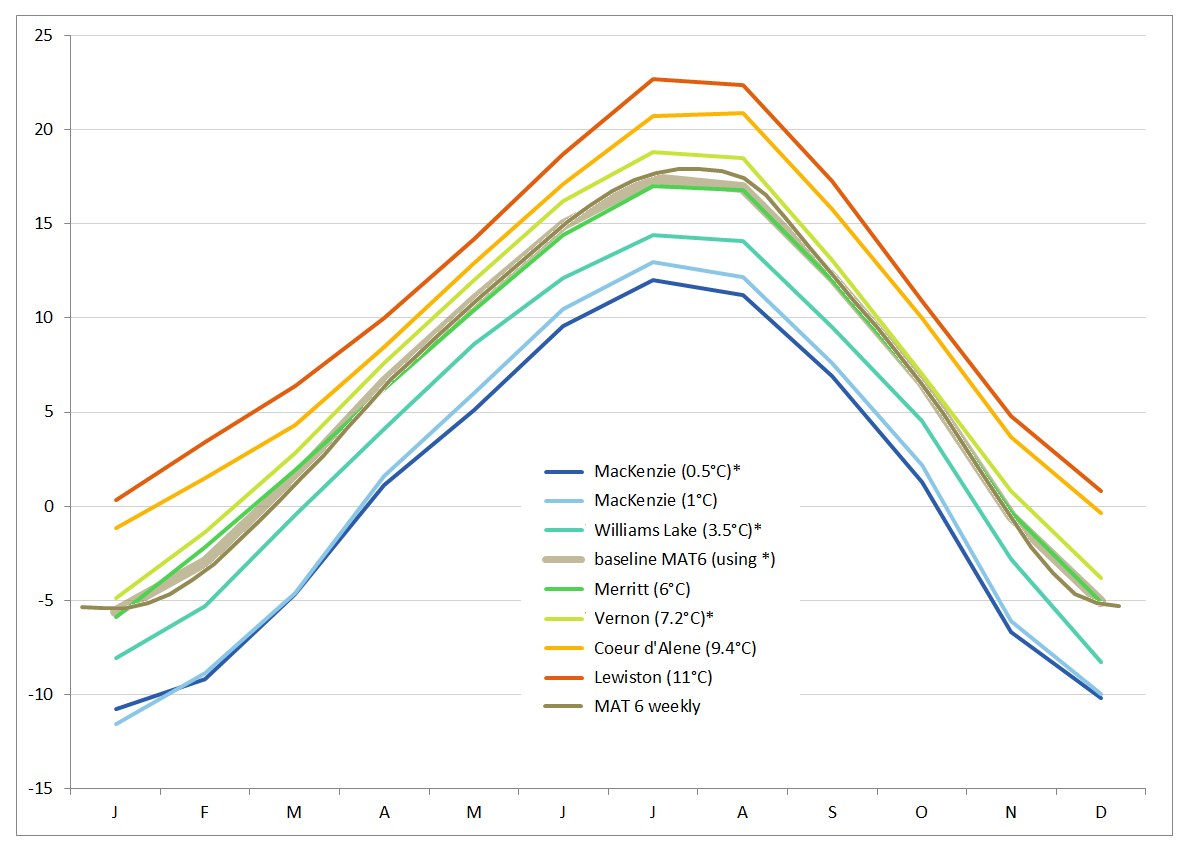
The choice of a point on the map representing your target climate is somewhat subjective, but there are reasons not to worry too much about this. Firstly, there is a similarity of patterns for locations in Western North America with continental climates, as indicated in the graph below. Secondly, we have always been more interested in the responses of genotypes relative to each other, rather than their absolute responses to the climate regimes. A third argument is that the averages affect plants far less than the extremes. Based on the monthly average temperatures obtained from ClimateBC for three chosen points on the map (indicated by *in the graph), a baseline curve was derived, and idealized curves can be derived by adding or subtracting a set number of degrees. The following graph shows how the (thick brown) baseline curve compares to several curves of real locations, as well as to the curve of weekly average temperatures (thin brown), which were obtained by interpolation.
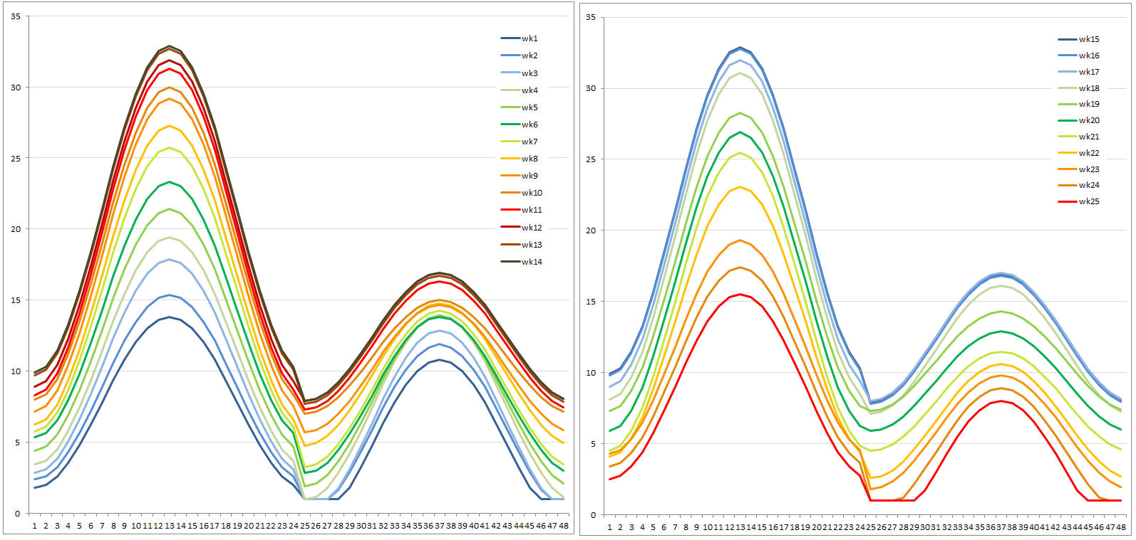
On this weekly temperature average, we superimpose a daily variation. Initially, we chose a daily range between 12 and 15 °C, which is representative for the three chosen climate points between April 15 and October 15, the period we chose to represent one growing season. In the field, sites with a mean annual temperature (MAT) between 4 and 5°C produce optimal growth for lodgepole pine (Wang et al. 20061). Warmer climates result in decreased growth. However, a similar set of lodgepole pine populations grown in controlled climate chambers under temperature regimes from 1 to 13°C (MAT) reveal neither plant stress nor decreased growth in the warmest regimes. Likely, there was not enough ‘weather’ in our simulated climates. This makes intuitive sense if we think about representing a climate of MAT 6 by programming a constant 6°C: this is not realistic. Neither is it realistic to keep the daily average and range nearly constant. Plants adjust to the higher average temperatures by permanent modifications in their physiology and metabolism, and deal with deviations from the averages through plasticity. When the capacity to adapt using a plastic response is exceeded, survival is at stake and differences in the ability to cope are revealed. The capacity of a plant to respond to stress will depend on the background signal of past average temperatures and extremes. Yet significant plant mortality leads to loss of data, so we try to avoid it. This is the fine line we are skirting when trying to make temperature regimes ‘realistic’. The way the climate is perceived by the plant is more important than the absolute values of temperatures. Yet we want to evaluate stress levels in terms of factors that have relevance in the field.
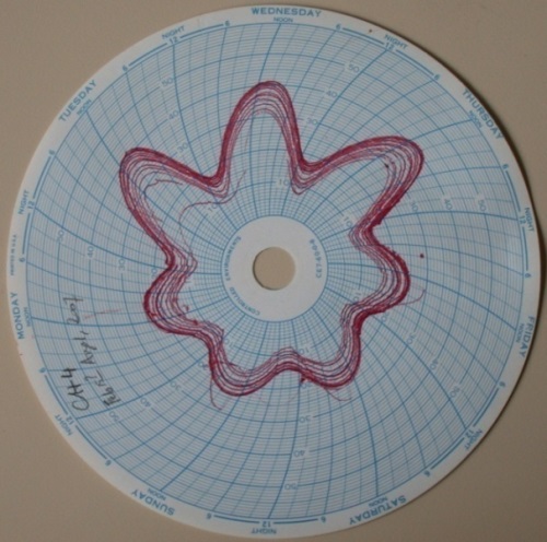
In a second iteration of the lodgepole pine experiment designed to produce response curves, the daily sinusoidal pattern, identical for all MAT, was overlaid on the seasonal trend in two alternating phases: a 3-day warm phase with large temperature variation, mimicking sunny days, and a 4-day cool phase with smaller diurnal fluctuations to mimic cloudy days. The analog temperature chart on the side gives a visual impression of these two phases for MAT13. Both diurnal range (between 8 and 23 °C) and daily average temperature were manipulated to achieve this goal. Weekly averages of temperature and daily range were maintained at their respective baselines. The result was a more realistic absolute maximum temperature in August of 35.4°C for MAT07. This is very close to 35.2°C, which is the absolute maximum in August in Vernon North weather station between 2006 and 2012. Indeed, absolute maximum temperature was the criterion around which the ranges were developed.
Extreme events play a large role in the response of plants to present and future climates. The background trend determines the pre-conditioning of the plants, and therefore the response to the extreme event. Both trends and extreme events need to be simulated carefully, close to the level of tolerance, to reveal differences in population response determining which populations survive and which ones don’t. Next I’ll cover moisture regimes.
Wang, T., A. Hamann, A. Yanchuk, G. A. O’Neill and S. N. Aitken. 2006. Use of response functions in selecting lodgepole pine populations for future climates. Global Change Biology 12: 2404–2416.