Pairs-Trading: Optimal Mean Reversion Strategy.

Recently much of my work has been revolving around building a trading strategy that optmises on the mean reverting behaviour of the stock market.

This blog post is to give insights into some of the interesting tools i have had the pleasure of working with.

Ornstein-Uhlenbeck process

$dX_t = \mu * (\theta - X_t) dt + \sigma dB_t$

with constants $\mu, \sigma > 0, \theta$ , and state space is in the Real domain. Here, B is a standard Brownian motion under P (historical probability measure), denote by $f_t$ $= F_{t>0}$ the filtration generated by X.

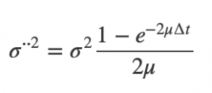
The parameter $\mu$ represents the equilibrium or mean value supported by fundamentals, $\sigma$ the degree of volatility around it caused by shocks and $\theta$ the rate by which these shocks dissipate and the variable reverts towards the mean.

Pairs Trading example

The pair of assets are selected to form a mean-reverting portfolio value. In addtion, one can adjust the strategy $(\alpha , \beta)$ to enhance the value of mean-reversion.
under the model.

with the constant

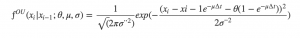
the conditional probability density of $X_t$ at $t_i$ given $x_{i-1}$ at $t_{i-1}$ with time increment.

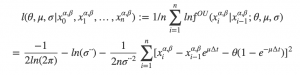
Maximising the average log-likelihood over $\theta,\mu \space$ and $\sigma$ for a given strategy $(\alpha, \beta)$ . For any $\alpha$ , we choose the strategy $(\alpha, \beta^*)$ , where ß is the argmax of the log likelihood equation.

think of $\alpha = B/S_0^{(2)}$ shares is held and at the same time we short $\beta = B/S_0^{(2)}$ shares in $S_0^{(2)}$ . This way the sign of the initial portfolio values depends on the sign of the difference A – B which is non- negative. Without loss of generality, we set A=1.

Log-likelihood function:

Using the observed $x_i$ , we maximise the average log-likelihood defined by.

Example
Using the price data from August 2011 to May 2012 (n = 200, ∆t = 1/252), for GLD-SLV and GLD-GDX.

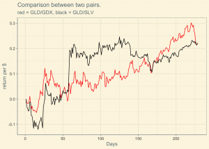
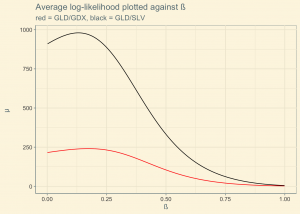
Shown above is the performance of a portfolio that has $\beta =1$ hence the equal ratio of spending is done in going long on GLD and shorting GDX (SLV).

The above chart shows the comparison between the two pairs trading examples using the optimised beta levels obtained through the use of the model.

Citations: Optimal Mean Reversion Trading with Transaction Costs and Stop-Loss Exit paper [Tim Leung and Xin Li.]

Leave a Reply Cancel reply