Possibly more important than our answer is our confidence in the answer. Our confidence is quantified by uncertainties as discussed earlier. Once we combine numbers, we need to be able to assess how the uncertainties change for the combination. This is called propagation of errors.
Error Types
- Mistakes
- Natural variation
- Systematic and random equipment problems
- Data collection methods
- Observer diligence
- Locations errors/accuracy
- Rasterizing and digitizing
- Mismatch of data collected by different methods (e.g., seafloor bathymetry)

Bathymetry of the Seafloor
Reliability Issues
- Changes in data over time
- Non-uniform coverage
- Map scales
- Observation density
- Sampling theorem (aliasing)
- Surrogate data and their relevance
- Round-off errors in computers
Error Propagation
Errors arise from data quality, model quality and data/model interaction.
We need to know the sources of the errors and how they propagate through our model.
Simplest representation of errors is to treat observations/attributes as statistical data – use mean and standard deviation.
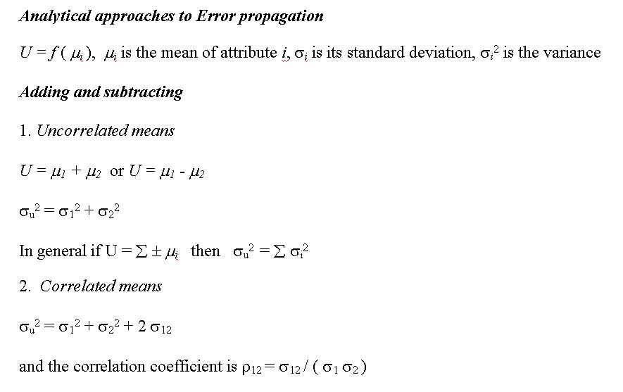
Addition and Subtraction
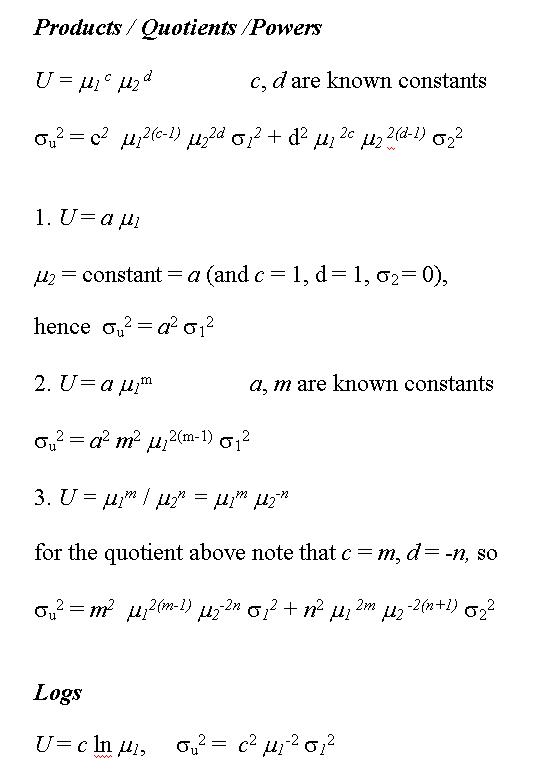
Multiplication, division, powers, logs
Monte Carlo Simulation
If a new attribute U is given by U = f (A1, A2, A3, …. An) where the A’s are attributes and f represents some function combining them, then we want to know what is the standard deviation of the combination U and how does the standard deviation of each A contribute to it?
By MC simulation we look at the statistical distribution of a lot of realizations (random samples) of U.
A single realization of U is Ui = f (R1, R2, R3, …. Rn) where each Rn is a random sample of its corresponding attribute An based on the statistical properties (mean and standard deviation, for example) of An. (At the end of these notes we show how to take a random sample of a distribution.) The probability functions for the attributes themselves need not be Gaussian and could even be taken from histograms of observed values.
The mean and standard deviation of U is estimated by
m= N-1 SUM i=1,N Ui
s2 = (N-1)-1 SUM i=1,N ( Ui – m)2
where N is a very large number of realizations (hundreds or thousands).
MC simulation is most useful when the function relating the attributes is complex or the statistical distribution is known only empirically (from a histogram, for example). For simpler combinations of attributes, there are easier, direct (analytical) ways to estimate the new uncertainties from the attribute uncertainties.
Notes on random number generation in Excel
For the Monte Carlo simulation, you will want to generate a series of random numbers with a normal (bell-curve) distribution. There are 2 ways to do this in Excel.
First, you can use the Tools > Data Analysis > Random number generation > Normal distribution to generate a sequence of random numbers.
Or, you can take advantage of the central limit theorem that states that under certain conditions, random samples of any distribution will have a normal distribution. The Excel function RAND generates a uniformly distributed random number, that is, the probability is the same for any number between 0 and 1 to be generated. To get a normally distributed random sample with mean of 0 and standard deviation of 1 we can simply add 12 uniformly distributed random numbers and subtract 6. To get a normally distributed random sample with mean of m and standard deviation of s we use:
[ SUMi=1,12 RAND ) – 6 ] * s + m
Because this expression is quite long in Excel you can create a macro to facilitate using it again and again. To record a macro, select Tools > Macro > Record new macro > give name to the macro > ok > type in expression > Stop recording. You can refer to re-named cells from within a macro, so you might want to use variable names for the mean and standard deviation to keep your macro general.
You can also specify a Control-key to run the macro from the worksheet. Otherwise, to run the macro, go to Tools > Macro > Macros > select the macro name and press Run.
Once the macro is run in a cell, you can drag the expression to other cells using the drag handle in the lower-right corner of the cell.
Statistical Tests
F-test: test if two distributions with the same mean are the same or different based on their variances and degrees of freedom.
T-test: test if two distributions with different means are the same or different based on their variances and degrees of freedom