Written by Paul Cote
Geographic information systems are information systems that permit complex associations to be made between entities using geometric references. In order to perform spatial associations, entities must be referenced in a common coordinate system. This statement seems obvious, however the problem of reconciling the coordinate systems of databases is a very important and common problem in GIS. There are hundreds of coordinate systems in common use, and each of these has valid justification. What prevents the establishment of a standard coordinate system for use in GIS is that the most useful coordinate systems are orthogonal (composed of axes that cross at right angles, and units that are equal in all parts of the grid) yet the earth is round and must be flattened to fit into an orthogonal coordinate system. There are many methods (projections) for making flat, orthogonal representations of the earth, but no single method will do a good job on the entire planet.
So, understanding coordinate systems — what their important qualities are, how to identify them and how to transform one into another, are very important skills for the educated GIS user. Even for the educated GIS patron, it is essential to have a critical understanding of the effect that improper — or even fully proper choices in coordinate systems may have on analysis.
Formal Coordinate System Concepts
Units
A referencing system must be capable of defining differences among entities. In a coordinate system, many differences are permitted to vary at the same time ('co' having a root meaning along the lines of 'with' , and 'ordinate' implying something to do with placement or measurement in some sort of scale). The incremental change that a coordinate system records are the units of measure. Because GIS data depends on recording and interpreting units, GIS data must be explicit in declaring what units are used.
Orthogonality
The most common sense of the word coordinate system assumes measurement within a grid defined by axes that meet at right angles, and unit scales that form parallel, continuous fields across a plane. The term orthogonal relates to the fact that at any location in the grid, the unit axes are meeting at right angles. Implied in this is that geometric relationships in one part of the grid can be compared with those in another part of the grid using simple plane geometry. Most GISystems rely on plane geometry for relating entities; therefore, they assume orthogonal coordinate systems.
Latitude and Longitude
The closest thing we have to a natural coordinate system for the earth; even so, there are many different schools of thought regarding how the degrees ought to be recorded. Latitude is measured in degrees north of the equator. The north pole is 90 degrees north. The south pole is 90 degrees south or -90 north. Longitude is measured in degrees east of Greenwich England. Boston is approximately 289 degrees east of Greenwich. Sometimes people say Boston is 71 degrees west, others may say that Boston is -71 degrees longitude. The parts of a degree are minutes (1/60th of a degree) and seconds (1/3600 of a degree, or 1/60th of a minute.) To make math easier, most GIS software will expect degrees, minutes and seconds to be converted to decimal degrees. When you have data with coordinates specified in degrees it may be referred to as 'Geographic Projection' or Unprojected. (Watch for 'natural' angular units that are often used in mathematics or statistical programs such as R that are not latitude or longitude--radians.)
Latitude and longitude are not orthogonal. The simplest illustration of this is that all of the meridians (north-south lines) meet at the poles. Thus, degrees of longitude are longer (in a plane geometric sense) at the equator than they are at other latitudes. This is why any geometric measurement other than 'is inside' or 'intersects' should be qualified by a statement of what coordinate system is being used.
Projections
Projections are methods of transforming latitude and longitude to planar, orthogonal. coordinate systems. There is no perfect way of doing this and, thus, a GIS user should expect to find data in any number of unexpected projected coordinate systems.
On-The-Fly Projection
Some software are capable of reconciling the data of different coordinate systems. If this works, it saves the user the trouble of converting the coordinate systems of the data (and perhaps having multiple versions of the same dataset.) Effectively, the software converts one coordinate system to the other when needed (or 'on-the-fly'). (Problem--ArcMap / ArcPro may still use the layer's 'internal' coordinate system when performing calculations and therefore the results may be incorrect [e.g., using degrees to calculate area].)
Forward on-the-fly Projection
This is one sort of on-the-fly projection which is only capable of converting from Latitude and Longitude to any number of 'target' projections.
Backward and Forward on-the-fly Projection
If you can convert from various projections into Latitude and longitude (backward projection), and from lat-lon into other projections (forward projection), then you basically can convert from one projected coordinate system to another.
Graphic Projection VS Computational Projection
Some software programs may profess to do on-the-fly projection, but before you trust them, make sure that the coordinate transformations are being used in calculations such as area and distance. Often, as is the case with ArcMap and ArcPro, orthogonal. coordinates are used for some functions but not all (e.g. the ReturnArea request.)
Coordinate System Transformations
We often need to express one geometric data set in the coordinate system of another. There are two basic problems, one is where the coordinate system of one of the data sets is unknown, and the other is when we know specific information about each of them.
Transforming geometry of an unknown coordinate system
When we have a rough map or an aerial photo with geometry that we would like to assimilate with other data in a GIS, we can begin by finding features on the foreign map that we know represent the same features on in the 'standard' coordinate system. We would call these common points 'Control Points' . We would call the coordinates of the foreign map x' and y' and the coordinates of the known coordinate system, x and y.
Coordinate Shift
By choosing one control point, we could transform our unknown geometry such that the entire coordinate system shifts, making the coordinates of that one point the same -- but probably failing to match anything else. This transformation can be defined as
y = y' + c
x = x' + d
Where c and d are constants
Scale, and Rotation
With two control points defined, a coordinate transformation is specified whereby a the foreign coordinate system is shifted, scaled and rotated such that a line on the foriegn system matches with a line in the GIS.
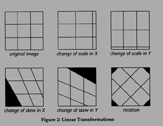
Skew
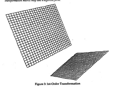
The two-point transformation given above will scale X and Y by the same factor, which is fine if we know that both coordinate systems have regular, orthogonal. units. With three control points picked we can align a triangle from the foreign geometry to a triangle in the GIS -- this may involve skewing or shearing the foreign geometry, effectively scaling x by a factor different than y. THis sort of transformation is known as an Affine transformation or sometimes a 'First Order Transform.'
An Affine transformation is described mathematically as:
x' = Ax + By + c
y'= Dx + Ey + f
(RMS) Errors of Fit
If you perform an affine transformation with more than three control points, an separate affine transformation can be attempted using all the possible triplets, then an average can be made that maximizes the 'Fit' of all the points. In this case, we might like to see an error report that reveals which points are not so cooperative to being realigned satisfactorily with an affine transformation. A good transformation interface will return root-mean-squared errors for each of the points. This RMS error is an estimation of the error for that particular point assuming that the transformation formula which was calculated is the correct one.
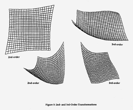
Higher Order Transformations (Warps)
An affine transformation can distort a planar coordinate system in all ways that preserve parallel lines, there are higher-order transformations which can through curves into our space. These are called higher-order transformations because the formulas for expressing x as a function of y' and x' are higher-order polynomials such as:
x = (y + c) * (x + d)
To make a long story short, the higher-order your polynomial, the more curvy your transformation can get.
- How much is too much? When transforming coordinate systems it is important to think about transformation the way we think about other associative functions in information systems -- that is we are trying to define a function that simulates the actual distortion of the geometry in the unknown system. There is a temptation to choose as many control points as possible and use the highest-order transformation to get the best fit for all of the points. But we should ask ourselves whether the distortion in our original is actually the result of such a regular function, or if perhaps, some of our control points are just not very good! My philosophy is that you most distorted cartographic hardcopy can be corrected well using a first-order transform. The secret is finding the correct points (or eliminating the bad ones). If you have an aerial photograph of terrain with a valley running down the middle of it, perhaps a second or third order transform is appropriate.
Rubber Sheeting
When a single warp method won't do the trick over an entire data set, one may want to 'morph' from one warp in one area to another warp in another corner of the data set. Using multiple transformations on a single geometric dataset is called rubber-sheeting.
Projection Transformation: The second type of problem in reconciling coordinate systems in datasets is where we have two coordinate systems which are different, but where the differences among them is mathematically understood from the beginning. To understand this, we need to understand the systematic ways that common map coordinate systems are created.
The dymaxion Projection Animation. Created by Christopher Rywalt.. A great exposition of an innovative projection designed by one of Harvard's most notable dropouts, Buckminster Fuller.
The most standard coordinate system for describing the geometry of things on planets like Earth is Latitude and Longitude (lat-lon). This coordinate system cannot logically be treated with normal coordinate system transformations as described above, because the axes are not orthogonal., and the units are not constant. A degree of longitude at the equator is much larger that a degree near one of the poles. The area of mathematics that deals with calculating geometric relationships in spherical coordinate systems like lat-lon is Geodesy the calculations involved in geodesy (spherical trigonometry) are much more complex than the plane trigonometry involved in rectangular coordinate systems, and most GIS products will not treat spherical coordinates correctly (although, if the area of analysis is small enough, the error may be negligible.)
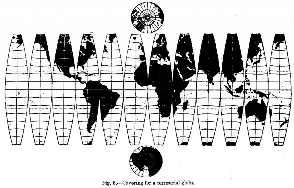
The problem of mapping the curved surface of the earth in a rectangular coordinate system has been explored for centuries. The process for doing this is called Map Projection. No map projection is perfect, the method used always involves distortion of some kind. Choosing the best projection for a particular application always involves a choice of which sort of distortion is going to represent the area of interest in the least harmful way.
The term Projection derives directly from the concept that a silhouette of any sort of object can be projected onto a flat surface (as with a light source and screen.) In the case of (very simple) map projection, the object is a transparent globe with geographic features drawn on it. When projected on a flat surface, the outlines of features on the curved surface become transferred in a systematic fashion to the flat screen.
This illustration (taken from Principals of Cartography by Erwin Raisz, published by McGraw Hill) illustrates the concept behind the Orthographic projection.
We have now overcome the round-earth problem, and we can overlay a rectangular coordinate system on our map. However, we should note that the coordinate system misrepresents the size of shapes near the edges of the globe. To be most accurate, the center of this projection (it's Point of Tangency) should always be at the center of our area of interest.
We could correct for the distortion in the size of objects represented near the edge by systematically widening the space between the meridians as we go out from the center -- as in this example of Lambert's Equal Area Projection.
In doing this we have ascended from our convenient analogy of a single light-source, to a process that is more difficult to diagram.
We now have two maps of one planet; each using a different projection system. We can lay the same coordinate grid on each of these projections, but we shouldn't be surprised when we find that identical places on the globe have different coordinates on the two maps. This is the reason that projection conversion is important.
Given that the systematic distortions of each projection system are known, along with such important Projection Parameters such as (in the case of an orthographic projection) The Projection's Center (its point of tangency), and coordinate system origin (its Datum,) are known, the locations differences in the coordinates between identical objects on the two maps can be described mathematically. Conversely, a map in one projection and coordinate system can be systematically transformed into another. Many good GIS products will convert among the hundreds of common projection systems provided the user can correctly specify the important projection parameters.
In GIS data, the use of orthographic projections is rare. The following illustration shows the three common variations on the concept of the flat projection screen.
A common variation on each of these takes off on the idea that the projection surface may intersect the surface of the globe (in technical parlance, the surface would be Secant, as opposed to tangent, with the sphere.)
The advantage of this, is that the area of nearly correct scale will be expanded. In the case of an orthographic projection a secant projection plane gives a circle of correct scale instead of a mere point. In cylindrical and conic projections, a secant projection surface yields 2 Standard Parallels instead of 1.
For each projection variant, a different set of projection parameters may be required in order to adequately specify a transformation method. Fortunately, cartographers have come to agreement on several standard projections that work best for different parts of the world. If you are lucky, or insightful enough to ask for it, data you obtain will come with the projection and coordinate system defined.
A Cylindrical Projection: The Mercator
The Mercator projection, invented by Gerardus Mercator (aka Gerardus Kremer) in 1569, is probably the most famous projection of all time. It is indisputably the best map projection for navigators because of its unique quality that an earth-bound traveler, following a line of constant compass direction, can chart her course on the mercator projection with a Straight Line. This quality was not accidental, Gerardus was a mathematics buff who used a logarithmic displacement of the parallels of latitude to obtain this effect as a service to navigators. It is said that Mercator was the first person to call a book an Atlas. In 1544 he was imprisoned for heresy, but released for lack of evidence.
Because the standard Mercator map is tangent to the Earth at the Equator, it represents size and scale only in lower attitudes, and grossly overestimates them near the poles. Consider that the north pole is actually a point, but in cylindrical projections it explodes to a line.
font size=3>The Universal Transverse Mercator Projection System
The most standard projection system for large-scale mapping projects (like the national map series produced by the U.S. Geological Survey, and the Ordinance Surveys of Britain and France) is a variation on the Mercator called the Universal Transverse Mercator (UTM. This projection overcomes the distortion problem inherent in the standard Mercator by simply putting the tangent line of the projection surface near the center of the area of interest.
The UTM system uses a Transverse version of the projection which is tangent along a meridian instead of the equator. There are 60 positions for this projection, dividing the planet into 60 zones. These zones guarantee that any place on earth can be no further than 3 degrees of longitude from a standard meridian. The UTM projection maintains the navigational convenience of the original design.
The Importance Metadata for Coordinate System and Projection Identification
The reconciliation of coordinate systems between maps and digital geographic data can at times involve a lot of guess-work, and can result in an unpredictable spatial mismatch of data that will impact the quality of your analysis, and could render all of your findings indefensible. There are ways of defending yourself against the insidious mystery of coordinate systems, however. The solution is metadata! If you are working with quality geographic information, and if you have foreseen the inevitable problems, you will have obtained, demanded, information about the coordinate system and projection used.