Interpolation Problem
A simple explanation of the interpolation problem (ignores commonly used functions such as inverse distance squared, however):
(Source: http://www4.ncsu.edu/~hmitaso/gmslab/viz/interp1d.html)
Five Different Surfaces
Surfaces created from the same data.
-
- TIN
-
- Topogrid
-
- Voronoi
-
- Kriging
-
- IDW
Source: Lubos Mitas and Helena Mitasova (http://www4.ncsu.edu/~hmitaso/gmslab/viz/sinter.html)
Inverse Distance Weights
The exponent associated with inverse distance weights determines how quickly the influence of neighbouring points drops off. With inverse distance, when trying to estimate an elevation (e.g.) at an unknown location, the weight (or significance) the interpolating routine gives to the elevation value at each known (sampled) location decays rapidly as the distance between the known and unknown points increases. How rapidly this occurs can be adjusted to best fit your real world situation by adjusting the value of the exponent. This graph illustrates the influence on inverse distance weighting for exponents 1 - 6. Note that you can use an exponent of less than 1, although that would give points further away a greater influence than nearer points! Typically weights of 1 or 2 are used.
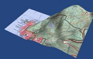
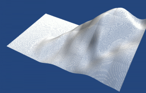
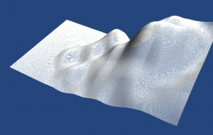
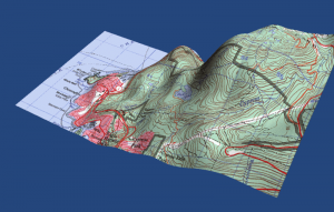
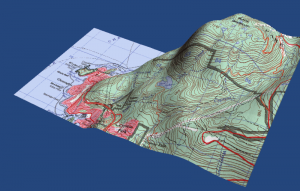
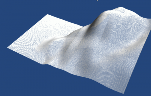
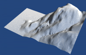
DEM Data Comparison
Below is a comparison of how different sources of DEM data--at different resolutions but for the same area--differ significantly in their representations (posted with permission of Dave Patton, original source: http://members.shaw.ca/davepatton/demcompare.html)
-
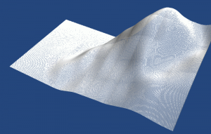
- Wireframe image using the SRTM 30 arc-second data, which is a “near-global digital elevation model (DEM) comprising a combination of data from the Shuttle Radar Topography Mission, flown in February, 2000 and the the U.S. Geological Survey’s GTOPO30 data set”.
-
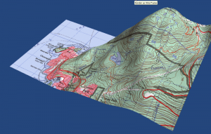
- Map image using the SRTM 30 arc-second data, which is a “near-global digital elevation model (DEM) comprising a combination of data from the Shuttle Radar Topography Mission, flown in February, 2000 and the the U.S. Geological Survey’s GTOPO30 data set”.
-
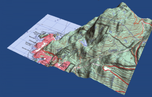
- Map image using the 3 arc-second SRTM (Shuttle Radar Topography Mission) North American data.
-
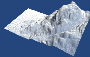
- Wireframe image using the 3 arc-second SRTM (Shuttle Radar Topography Mission) North American data.
-
- Map image using the 30 arc-second GTOPO30 data.
-
- Wireframe image using the 30 arc-second GTOPO30 data.
-
- Wireframe image using the GLOBE 30 arc-second data.
-
- Map image using the GLOBE 30 arc-second data.
-
- Map image using the NIMA (now called NGA) 30 arc-second DTED Level 0 data.
-
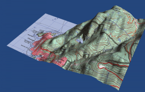
- Map image using the 3 arc-second GeoBase Canadian Digital Elevation Data Level 1 DEM at 1:250,000 scale.
-
- Wireframe image using the NIMA (now called NGA) 30 arc-second DTED Level 0 data.GLOBE 30 arc-second
-
- Wireframe image using the 3 arc-second GeoBase Canadian Digital Elevation Data Level 1 DEM at 1:250,000 scale.
-
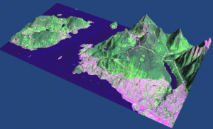
- Part of a satellite image from the GeoGratis Landsat-7 Orthorectified Imagery over Canada, using the 0.75 arc-second GeoBase Canadian Digital Elevation Data Level 1 DEM at 1:50,000 scale.
-
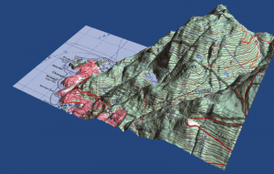
- Map image using the 0.75 arc-second GeoBase Canadian Digital Elevation Data Level 1 DEM at 1:50,000 scale.
-
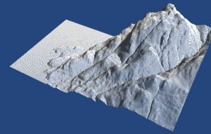
- Wireframe image using the 0.75 arc-second GeoBase Canadian Digital Elevation Data Level 1 DEM at 1:50,000 scale.
Areal Interpolation
Download this presentation by Dr. Waldo Tobler--the person who developed pycnophylactic interpolation or reallocation.
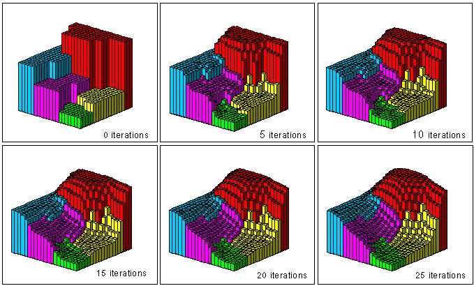
Pycnophylactic Interpolation
A simple graphic example of pycnophylactic interpolation (note how the transitions between the areal units becomes smoother, and also how the volume within each areal unit remains constant [i.e., if some of the blocks within an area get taller, others will get shorter to compensate]).