06/3/14

Simulating climates in growth chambers – Choosing day length regimes

This post is part of the series Simulating Climates in Growth Chambers.

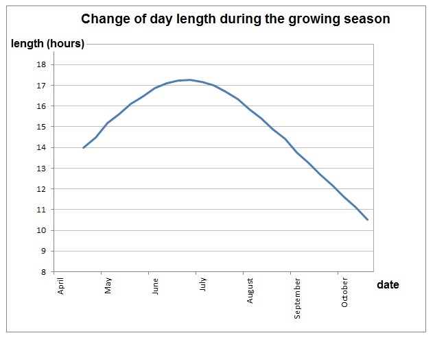
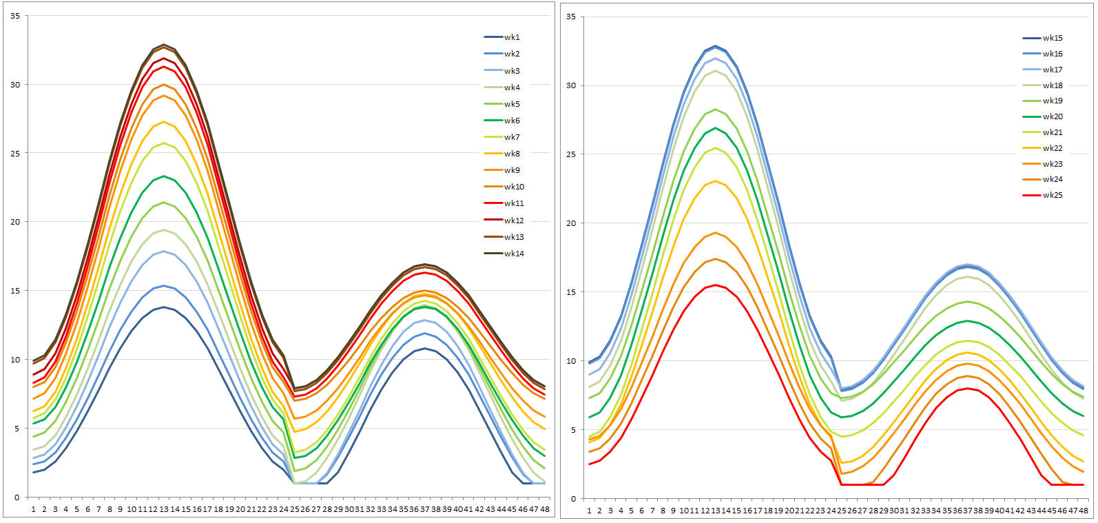
Day length for a given latitude can be obtained from online programs, such as the online photoperiod calculator at http://www.sci.fi/~benefon/sol.html Day length was reprogrammed weekly for convenience. Latitude can be chosen corresponding to a target location (e.g., Williams Lake, 52°07’N) or latitude representative of an area, e.g. the province of B.C. (54.5°N).

Some practical limitations may rise here. Until LED lights become cheaper still, any light source also generates heat. It may not be possible to program a sunrise while temperatures are still below 4°C. This depends on the hardware of the climate chamber. In this case, consider turning on the lights gradually, reducing light intensity, and leaving off any incandescent lights until later, as they generate a relatively high percentage of heat.

Next up on the list is simulating winter conditions, heat waves, stimulating germination and bud set. You can also go back through some of our older posts on simulating climates in growth chambers.

 Day length during the growing season at 54.5 °N.

Day length during the growing season at 54.5 °N.

06/2/14

Simulating climates in growth chambers – Developing moisture regimes

This post is part of the series Simulating Climates in Growth Chambers.

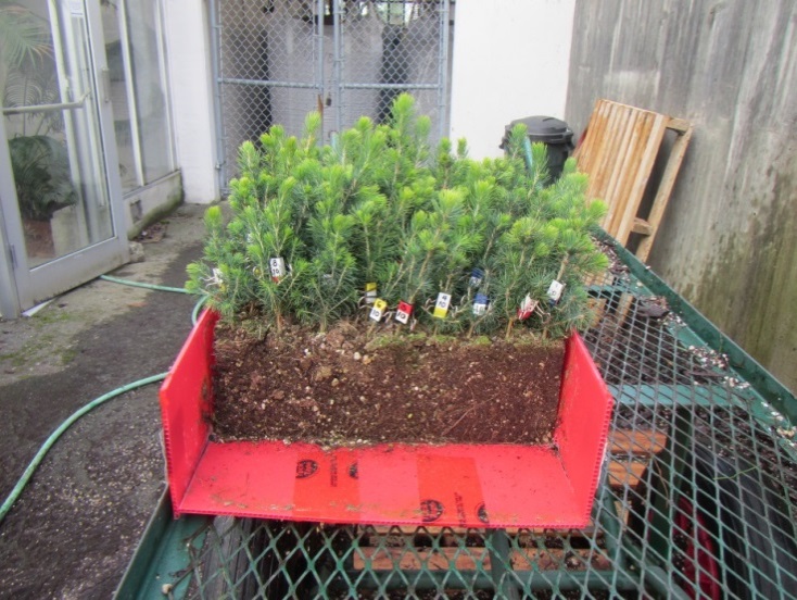
In continental North-West America, summer heat is correlated with drought. To make our climates more realistic, we added drought treatments. The simplest way to do this is subject plants in a ‘dry treatment’ to drought cycles, with soil moisture content dropping to 25% relative to total saturation1, before plants are re-supplied with water and fertilizer. In the ‘wet’ treatment, soil moisture content is maintained above 65% relative to saturation. Wet and dry treatments receive the same amount of fertilizer2. In order to apply drought treatments consistently, we use boxes of 40×36 cm where 100 plants share the same soil volume (15.8 l). This circumvents the problem of larger plants being more drought-stressed, as can happen when using individual plant cones. The boxes are made from Coroplast, a plastic corrugated cardboard, which can easily be cut with an Exacto knife. This allows us to size the boxes exactly the way we want them, and optimally use the space in the growth chamber.

Plant box opened on the side with the plants tagged for root washing

Plant box opened on the side with the plants tagged for root washing

As with using individual containers, planting distance needs to be balanced against experiment duration, chosen climate and resulting expected plant size, unless mortality due to plant competition is desired. However, too low a plant density will result in very few and long drought cycles, smaller treatment effects, reduced opportunities to fertilize, and possibly malnutrition. If you need to separate the plants at the end of the experiment, check out this blog post to find out how we avoided the problem of the roots becoming too entangled.

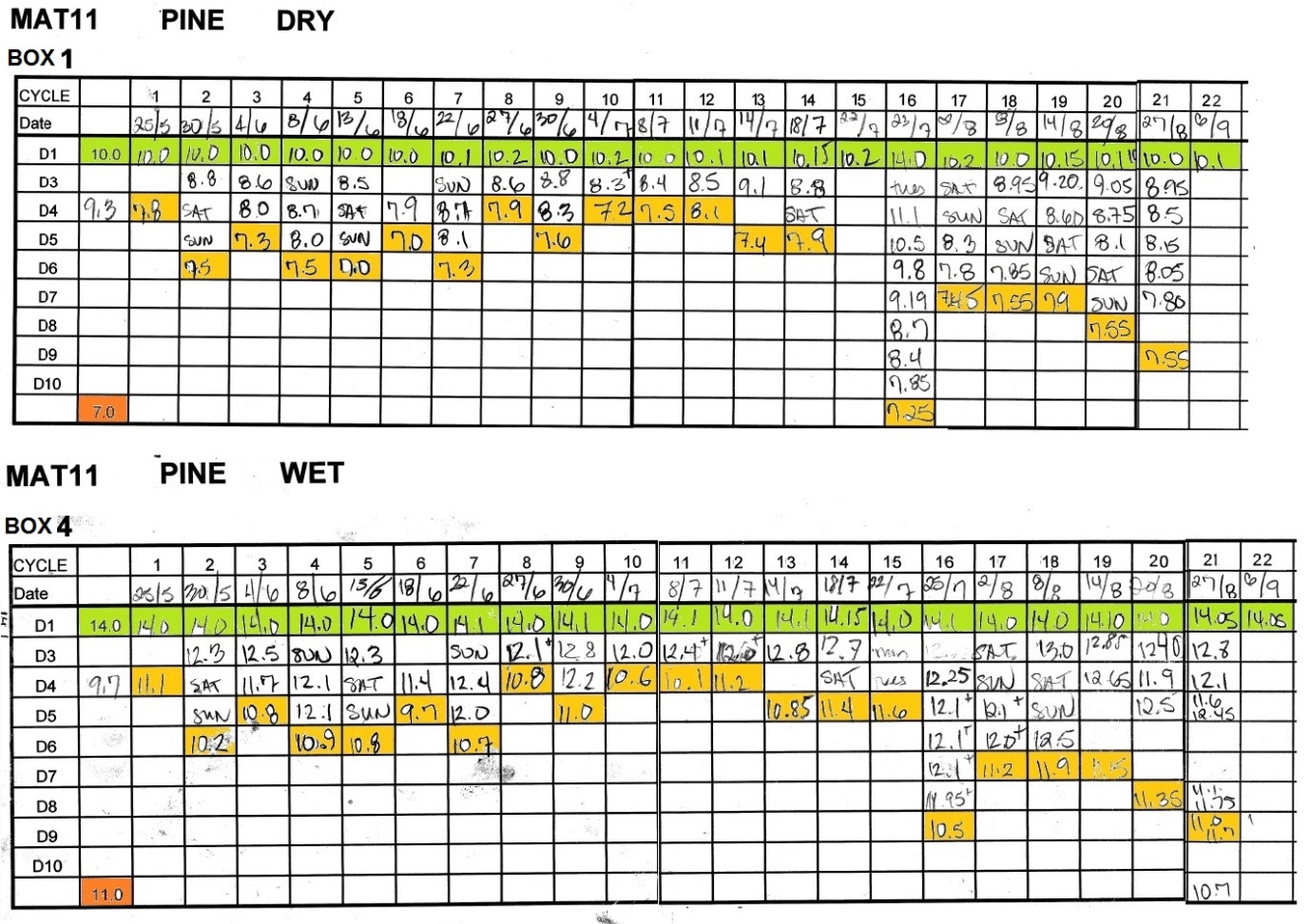
Example of box weights for dry and wet treatments. The first column indicates the target maximum and minimum weights. All wet and all dry boxes are fertilized at the same time, hence individual box weights may differ slightly from the target

Example of box weights for dry and wet treatments. The first column indicates the target maximum and minimum weights. All wet and all dry boxes are fertilized at the same time, hence individual box weights may differ slightly from the target

Come back tomorrow to find out how I applied day length regimes or go back and see some of the other posts in the series.


1 This is a point we previously established for the given soil mix to correspond to a soil water potential of -1 MPa, the point at which permanent damage starts to occur.

2 That is, at the end of each drought cycle and in comparative amounts (topping up with water if needed).

06/1/14

Simulating climates in growth chambers – Developing temperature regimes

This post is part of the series Simulating Climates in Growth Chambers.

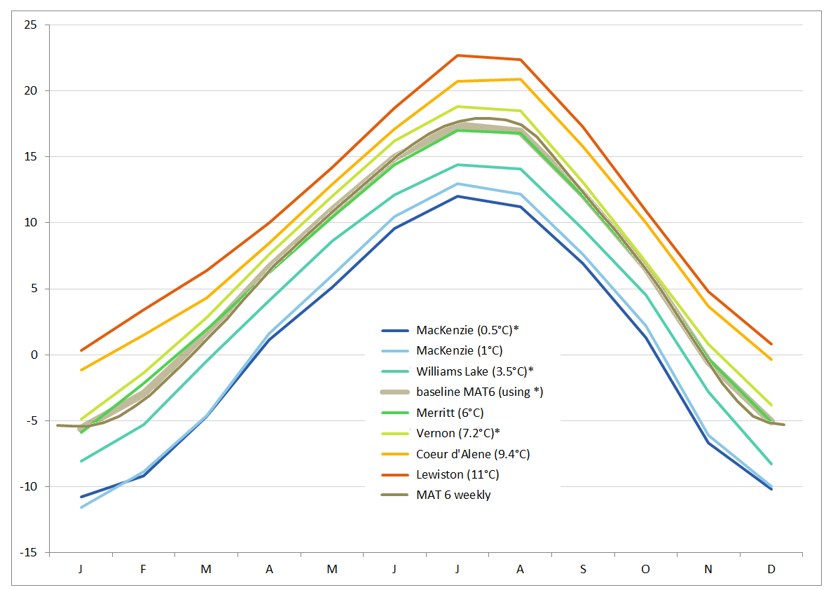
The choice of a point on the map representing your target climate is somewhat subjective, but there are reasons not to worry too much about this. Firstly, there is a similarity of patterns for locations in Western North America with continental climates, as indicated in the graph below. Secondly, we have always been more interested in the responses of genotypes relative to each other, rather than their absolute responses to the climate regimes. A third argument is that the averages affect plants far less than the extremes. Based on the monthly average temperatures obtained from ClimateBC for three chosen points on the map (indicated by *in the graph), a baseline curve was derived, and idealized curves can be derived by adding or subtracting a set number of degrees. The following graph shows how the (thick brown) baseline curve compares to several curves of real locations, as well as to the curve of weekly average temperatures (thin brown), which were obtained by interpolation.

Monthly average temperatures for seven locations in Western North America with continental climates, baseline curve for MAT 6 °C, and weekly averages interpolated from the baseline.

Monthly average temperatures for seven locations in Western North America with continental climates, baseline curve for MAT 6 °C, and weekly averages interpolated from the baseline.

On this weekly temperature average, we superimpose a daily variation. Initially, we chose a daily range between 12 and 15 °C, which is representative for the three chosen climate points between April 15 and October 15, the period we chose to represent one growing season. In the field, sites with a mean annual temperature (MAT) between 4 and 5°C produce optimal growth for lodgepole pine (Wang et al. 20061). Warmer climates result in decreased growth. However, a similar set of lodgepole pine populations grown in controlled climate chambers under temperature regimes from 1 to 13°C (MAT) reveal neither plant stress nor decreased growth in the warmest regimes. Likely, there was not enough ‘weather’ in our simulated climates. This makes intuitive sense if we think about representing a climate of MAT 6 by programming a constant 6°C: this is not realistic. Neither is it realistic to keep the daily average and range nearly constant. Plants adjust to the higher average temperatures by permanent modifications in their physiology and metabolism, and deal with deviations from the averages through plasticity. When the capacity to adapt using a plastic response is exceeded, survival is at stake and differences in the ability to cope are revealed. The capacity of a plant to respond to stress will depend on the background signal of past average temperatures and extremes. Yet significant plant mortality leads to loss of data, so we try to avoid it. This is the fine line we are skirting when trying to make temperature regimes ‘realistic’. The way the climate is perceived by the plant is more important than the absolute values of temperatures. Yet we want to evaluate stress levels in terms of factors that have relevance in the field.

Introduction of two alternating phases.

Introduction of two alternating phases.

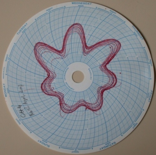
In a second iteration of the lodgepole pine experiment designed to produce response curves, the daily sinusoidal pattern, identical for all MAT, was overlaid on the seasonal trend in two alternating phases: a 3-day warm phase with large temperature variation, mimicking sunny days, and a 4-day cool phase with smaller diurnal fluctuations to mimic cloudy days. The analog temperature chart on the side gives a visual impression of these two phases for MAT13. Both diurnal range (between 8 and 23 °C) and daily average temperature were manipulated to achieve this goal. Weekly averages of temperature and daily range were maintained at their respective baselines. The result was a more realistic absolute maximum temperature in August of 35.4°C for MAT07. This is very close to 35.2°C, which is the absolute maximum in August in Vernon North weather station between 2006 and 2012. Indeed, absolute maximum temperature was the criterion around which the ranges were developed.

Daily temperatures on day 3 and 4 of the week. Each day represents one of the two alternating phases (warm sunny days and cool cloudy days) introduced to render the growing regimes more realistic. Left: gradually increasing temperatures during spring. Right: gradually decreasing temperatures from July 15 onwards.

Daily temperatures on day 3 and 4 of the week. Each day represents one of the two alternating phases (warm sunny days and cool cloudy days) introduced to render the growing regimes more realistic. Left: gradually increasing temperatures during spring. Right: gradually decreasing temperatures from July 15 onwards.

Extreme events play a large role in the response of plants to present and future climates. The background trend determines the pre-conditioning of the plants, and therefore the response to the extreme event. Both trends and extreme events need to be simulated carefully, close to the level of tolerance, to reveal differences in population response determining which populations survive and which ones don’t. Next I’ll cover moisture regimes.


Wang, T., A. Hamann, A. Yanchuk, G. A. O’Neill and S. N. Aitken. 2006. Use of response functions in selecting lodgepole pine populations for future climates. Global Change Biology 12: 2404–2416.

06/1/14

Climate vs. Weather: the why and how of simulating climates in growth chambers

This is the first in a series of posts on simulating climates in growth chambers. See the end of this post for a full list of entries in this series.

Our lab group investigates genetic variation that is meaningful to local adaptation, with a focus on trees. This is especially important in the context of climate change: long-lived trees may become maladapted over time to the local climate. To what extent are trees locally adapted, and to what extent does plasticity enable them to deal with a variety of circumstances? Valuable information is provided by long-term “provenance trials” in the field and nursery-type “common gardens”, in which a collection of genotypes from various sources is grown in the same environment, or set of environments. The weather in such environments varies from year to year and is not under our control. Over a longer term, the impact of this varying weather is expected to average out and represent the local climate. Yet there will always be some extreme event, perhaps an unusually late spring frost, a summer heat wave, a prolonged drought, or perhaps a very wet rainy season, which affects growth and survival in field trials. And these extreme events have a large effect on ‘adaptation’ in the genetic sense: natural selection for fitness.

WHY ?

Wishing to free ourselves from the vagaries of weather and to test our plant materials in warmer environments than those presently available in the field, we arrive at the controlled climate chamber. There are many restrictions inherent in using growth chambers. They are expensive. Only a limited number of genotypes can be observed over a short period of time. And simulating realistic winters has so far eluded us. This method should be regarded as complementary to field trials, and not a substitute.

HOW ?

How does one go about programming a controlled climate chamber to achieve a set goal? Which temperatures, light intensities and day lengths do we program? From which data set do we derive relevant climate variables, which are those variables, what range do we wish to cover, and is the resulting program actually realistic?

Choosing a baseline data set

We use data from Canadian Climate Normals of 1961-1990, the earliest data set of sufficient coverage and detail.This represents the climate before significant warming occurred, and it is the climate we assume the trees have adapted to through natural selection.

Choosing relevant climate variable(s) and a range you wish to cover

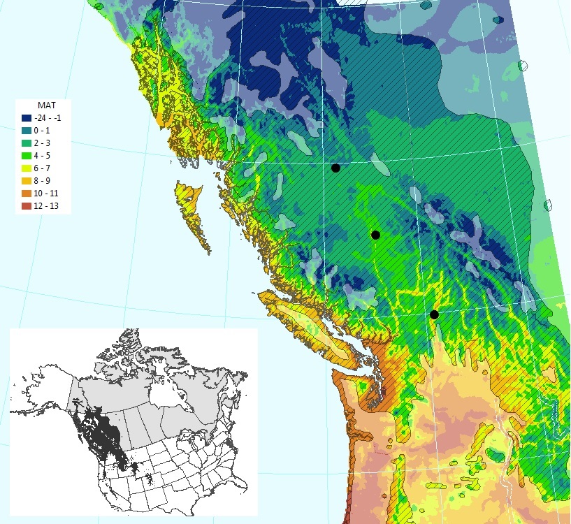
In our first experiments we studied interior lodgepole pine (Pinus contorta ssp. latifolia) populations. For this species, mean annual temperature (MAT) of the seed source is the variable revealing the strongest patterns of correlation with growth (Wang et al. 2006). ClimateWNA (Wang et al. 2012) data were used to plot the map of MAT below.

Natural range of Pinus contorta in North America (insert, dark grey) and detail of climate conditions (MAT, °C) in the area of interest (British Columbia, excluding the milky-white overlay where the species does not occur). Three chosen locations with representative climates (black dots).

Natural range of Pinus contorta in North America (insert, dark grey) and detail of climate conditions (MAT, °C) in the area of interest (British Columbia, excluding the milky-white overlay where the species does not occur). Three chosen locations with representative climates (black dots).

Our range of interest was interior British Columbia (BC), MAT 1 to 10 °C, to fully capture the growth response functions derived from field data (Wang et al. 2006). The geographic range for ssp. latifolia does not incorporate any areas with MAT 10°C, so this warmer, future climate regime was created by extrapolation. No attempt was made to average the climate for all the points with the same MAT. Instead, three points were chosen on the map, with MAT close to 1, 4 and 7°C, which had weather stations nearby. Such proximity is not really required, since ClimateWNA also provides detail on average daily ranges, but is still useful to inform us about the absolute maximum temperature. Other species may require other approaches, depending on the climate variables that best explain their adaptation. Now that a target climate has been chosen, find out how I developed realistic temperature regimes, moisture regimes, and where you can find suitable photoperiod data. Over the next several days, we’ll be posting on simulating winter conditions, heat waves, stimulating germination and bud set. At the end of the story, you will be familiar with most of the methods we had to use for growing plants for our AdapTree project. If you have tried similar or even stranger things, let me know. I’m curious to find out!

Simulating climates in growth chambers

Note: entries in this list will become available as posts go live between June 1 and June 8


Wang, T., A. Hamann, A. Yanchuk, G. A. O’Neill and S. N. Aitken. 2006. Use of response functions in selecting lodgepole pine populations for future climates. Global Change Biology 12: 2404–2416. Wang, T., A. Hamann, D.L. Spittlehouse and T. Murdock. 2012. ClimateWNA – High-Resolution Spatial Climate Data for Western North America. Journal of Applied Meteorology and Climatology, 51: 16-29.

04/2/14

Lodgepole pine DNA extractions

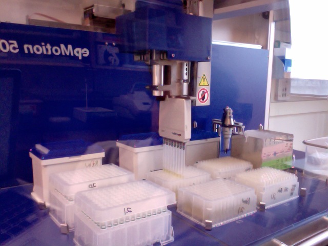
If you’ve read any of my previous posts, you may be aware that I have a truck-load of lodgepole pine samples collected last summer that are destined for SNP genotyping in the near future. I am close to wrapping up all of my DNA extractions (fingers crossed) for sending out, and because I tinkered a bit with the standard extraction protocol, I thought I’d discuss it here. Before I get there though, I have to give huge, gigantic, endless thanks to Kristin Nurkowski and Robin Mellway for all of their help. Most of these adjustments are a direct result of their insight and suggestions. They also taught me the standard protocol, how to use the lab’s robot, and saw me through lots and lots of troubleshooting.

To start at the beginning, I have needle samples collected on silica gel. In the field, my assistants and I tried to take the freshest tissue possible (new needle growth at branch ends), which was then kept on silica gel in coin envelopes within sealed ziplocs. When it was not possible to collect new needles, older ones were taken, and we even sampled some clearly dead trees (brown needles) in the off chance they’d work and some dying trees (recently fallen tree, needles not yet brown and brittle, but clearly dead); I’ll discuss this again a bit later. My collections in the Yukon were much later in the summer, so new growth was not new anymore, and we ran into a couple rainy days here which is a real pain when storing on silica. Other notable points were that these samples then sat in tupperwares in the back of a truck for at most 2 weeks while we continued collecting, so they definitely experienced some warm temperatures, but I have seen no correlation in the time since collection and the quality of DNA.
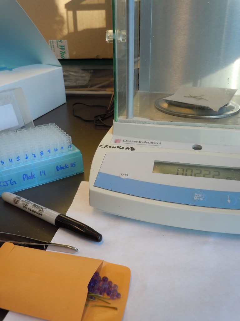
For the standard extraction, we used Machery-Nagel kits with NucleoSpin filters. These come with two different protocols using either PL1 lysis buffer or PL2 lysis buffer. From an initial test of both protocols and various weights of tissues, I found for my samples that the PL2 protocol worked better. PL1 is based on a CTAB extraction while PL2 is SDS based and has an additional step of a protein precipitation using potassium acetate (PL3). 20mg of tissue (dried) also seemed to be best, with less not giving enough DNA, and more also decreasing in yield. Presumably one could increase the amounts of buffers and reagents used per reaction relative to increase in tissue if more tissue wanted to be used, but at these volumes the filters were filled quite high with supernatant at the binding step, so eventually there is a limit. Except where I have pointed out exceptions, I followed the protocol outlined in the manual and used the volumes given, and just upped my lysis incubation to 45 minutes at 65C and my protein precipitation to 20 minutes at -20C (on ice, and in the freezer).

Initially I stuck with this protocol and it worked well.  I had about 80% success per plate, which I was pleased with considering the quality of some of my tissue samples. And believe it or not, some of the dead needles we had collected yielded DNA with enough to meet the cutoff! After completing eight plates of extractions, we had some issues crop up with our robot, and then extractions after that started failing. It is unclear if it was a product of the robot or a bad set of reagents or something entirely unknown, but it was clear nothing in the protocol had changed. It was also clear that it was not alone due to the quality of samples being used as some were trees from the same sites and provenances as samples that had already worked successfully. I did a lot of troubleshooting at this point to try to get things back up and running and eventually we found that adding PVPP to the PL2 buffer got us back up to an 80% success rate.

I used a 1% PVPP buffer for a while and then increased to 2% which improved it further. Because PVPP is mainly insoluble in liquid, I didn’t see the point in increasing past this as it was clear that there was undissolved PVPP in my buffer. I added 1 gram of PVPP to 50 mL of the PL2 buffer (preheated at 65C) plus 10 ul of antifoaming agent since the PL2 is quite bubbly, and incubated this overnight at 65C with 1 mL of RNaseA being added just before starting the extraction. A shaking incubator might be nice to use here since in the water bath, a lot of the PVPP just settles at the bottom of the tube. Using the PVPP improved my 260/230 from about 1.75 on average before to 2.33 on average.

Additionally, it seemed that the second plate from each extraction was on average coming out with poorer quality — the robot can do two plates at once. The robot is not incredibly fast at pipetting, so with a second plate, it sits there a little longer than the first before it is acted upon. This can be helped in the beginning by not removing the second plate of ground tissue from the freezer until just when the robot is ready to add lysis buffer to it. Because I did not have a very large number of plates to do, I instead began single plate extractions and simply kept an old used plate, filter, and elution plate to balance the centrifuge at the necessary steps. It is worth pointing out here that this was not the most efficient route. Though I have not raced the robot, if I had had access to a multichannel pipette, it is clear that doing this protocol sans robot would have been faster and easier. The robot is by no means a requirement for this extraction protocol, but it does have the added benefit of freeing you up to do other work while it pipettes away. I have even heard that newer models of robots have arms that will move the plates around for you! And the robot will definitely be a huge help for the plate normalization step once I have all my samples.
Some final points to make for anyone following along: from nanodropping my samples and qubiting a subset of them, most had about 40% less DNA per ul than was shown by the nanodrop, and I found no significant correlation of this with either my 260/230 or 260/280, though others in the lab have found that to be related for samples extracted from fresh, frozen tissue under the PL1 protocol, and with less of a decrease in DNA quantity between the two.

For samples that didn’t meet my cutoff criteria in terms of quality and quantity, performing the same extraction protocol a second time was successful about 60% of the time. I would speculate that the first failure in these cases was due to either the robot picking up some of the pellet with the supernatant which happened on rare occasions, or due to differences between different needles collected from the same tree.

And lastly, for those samples that did not succeed the first or second time around, it is now time to perform the more labor-intensive but hopefully cleaner and higher-yielding CTAB extraction protocol! Most of my samples that fall into this category are those I collected from the Yukon, so a product of the tissue being older and additionally not drying as quickly from the rainy day extractions. So for anyone out there planning a field season, I definitely advise lots and lots of extra silica gel and the youngest tissue possible — two already-well-known points that cannot be emphasized enough. If I have any serious alterations to the CTAB protocol, I may update this post or add another, but until then I hope that some of this information might be useful to anyone else out there working with conifers and their pesky secondary compounds!