06/3/14

Simulating climates in growth chambers – Choosing day length regimes

This post is part of the series Simulating Climates in Growth Chambers.

Day length for a given latitude can be obtained from online programs, such as the online photoperiod calculator at http://www.sci.fi/~benefon/sol.html Day length was reprogrammed weekly for convenience. Latitude can be chosen corresponding to a target location (e.g., Williams Lake, 52°07’N) or latitude representative of an area, e.g. the province of B.C. (54.5°N).

Some practical limitations may rise here. Until LED lights become cheaper still, any light source also generates heat. It may not be possible to program a sunrise while temperatures are still below 4°C. This depends on the hardware of the climate chamber. In this case, consider turning on the lights gradually, reducing light intensity, and leaving off any incandescent lights until later, as they generate a relatively high percentage of heat.

Next up on the list is simulating winter conditions, heat waves, stimulating germination and bud set. You can also go back through some of our older posts on simulating climates in growth chambers.

Day length during the growing season at 54.5 °N.

06/2/14

Simulating climates in growth chambers – Developing moisture regimes

This post is part of the series Simulating Climates in Growth Chambers.

In continental North-West America, summer heat is correlated with drought. To make our climates more realistic, we added drought treatments. The simplest way to do this is subject plants in a ‘dry treatment’ to drought cycles, with soil moisture content dropping to 25% relative to total saturation¹, before plants are re-supplied with water and fertilizer. In the ‘wet’ treatment, soil moisture content is maintained above 65% relative to saturation. Wet and dry treatments receive the same amount of fertilizer². In order to apply drought treatments consistently, we use boxes of 40×36 cm where 100 plants share the same soil volume (15.8 l). This circumvents the problem of larger plants being more drought-stressed, as can happen when using individual plant cones. The boxes are made from Coroplast, a plastic corrugated cardboard, which can easily be cut with an Exacto knife. This allows us to size the boxes exactly the way we want them, and optimally use the space in the growth chamber.

Plant box opened on the side with the plants tagged for root washing

As with using individual containers, planting distance needs to be balanced against experiment duration, chosen climate and resulting expected plant size, unless mortality due to plant competition is desired. However, too low a plant density will result in very few and long drought cycles, smaller treatment effects, reduced opportunities to fertilize, and possibly malnutrition. If you need to separate the plants at the end of the experiment, check out this blog post to find out how we avoided the problem of the roots becoming too entangled.

Example of box weights for dry and wet treatments. The first column indicates the target maximum and minimum weights. All wet and all dry boxes are fertilized at the same time, hence individual box weights may differ slightly from the target

Come back tomorrow to find out how I applied day length regimes or go back and see some of the other posts in the series.

1 This is a point we previously established for the given soil mix to correspond to a soil water potential of -1 MPa, the point at which permanent damage starts to occur.

2 That is, at the end of each drought cycle and in comparative amounts (topping up with water if needed).

06/1/14

Simulating climates in growth chambers – Developing temperature regimes

This post is part of the series Simulating Climates in Growth Chambers.

The choice of a point on the map representing your target climate is somewhat subjective, but there are reasons not to worry too much about this. Firstly, there is a similarity of patterns for locations in Western North America with continental climates, as indicated in the graph below. Secondly, we have always been more interested in the responses of genotypes relative to each other, rather than their absolute responses to the climate regimes. A third argument is that the averages affect plants far less than the extremes. Based on the monthly average temperatures obtained from ClimateBC for three chosen points on the map (indicated by *in the graph), a baseline curve was derived, and idealized curves can be derived by adding or subtracting a set number of degrees. The following graph shows how the (thick brown) baseline curve compares to several curves of real locations, as well as to the curve of weekly average temperatures (thin brown), which were obtained by interpolation.

Monthly average temperatures for seven locations in Western North America with continental climates, baseline curve for MAT 6 °C, and weekly averages interpolated from the baseline.

On this weekly temperature average, we superimpose a daily variation. Initially, we chose a daily range between 12 and 15 °C, which is representative for the three chosen climate points between April 15 and October 15, the period we chose to represent one growing season. In the field, sites with a mean annual temperature (MAT) between 4 and 5°C produce optimal growth for lodgepole pine (Wang et al. 20061). Warmer climates result in decreased growth. However, a similar set of lodgepole pine populations grown in controlled climate chambers under temperature regimes from 1 to 13°C (MAT) reveal neither plant stress nor decreased growth in the warmest regimes. Likely, there was not enough ‘weather’ in our simulated climates. This makes intuitive sense if we think about representing a climate of MAT 6 by programming a constant 6°C: this is not realistic. Neither is it realistic to keep the daily average and range nearly constant. Plants adjust to the higher average temperatures by permanent modifications in their physiology and metabolism, and deal with deviations from the averages through plasticity. When the capacity to adapt using a plastic response is exceeded, survival is at stake and differences in the ability to cope are revealed. The capacity of a plant to respond to stress will depend on the background signal of past average temperatures and extremes. Yet significant plant mortality leads to loss of data, so we try to avoid it. This is the fine line we are skirting when trying to make temperature regimes ‘realistic’. The way the climate is perceived by the plant is more important than the absolute values of temperatures. Yet we want to evaluate stress levels in terms of factors that have relevance in the field.

Introduction of two alternating phases.

In a second iteration of the lodgepole pine experiment designed to produce response curves, the daily sinusoidal pattern, identical for all MAT, was overlaid on the seasonal trend in two alternating phases: a 3-day warm phase with large temperature variation, mimicking sunny days, and a 4-day cool phase with smaller diurnal fluctuations to mimic cloudy days. The analog temperature chart on the side gives a visual impression of these two phases for MAT13. Both diurnal range (between 8 and 23 °C) and daily average temperature were manipulated to achieve this goal. Weekly averages of temperature and daily range were maintained at their respective baselines. The result was a more realistic absolute maximum temperature in August of 35.4°C for MAT07. This is very close to 35.2°C, which is the absolute maximum in August in Vernon North weather station between 2006 and 2012. Indeed, absolute maximum temperature was the criterion around which the ranges were developed.

Daily temperatures on day 3 and 4 of the week. Each day represents one of the two alternating phases (warm sunny days and cool cloudy days) introduced to render the growing regimes more realistic. Left: gradually increasing temperatures during spring. Right: gradually decreasing temperatures from July 15 onwards.

Extreme events play a large role in the response of plants to present and future climates. The background trend determines the pre-conditioning of the plants, and therefore the response to the extreme event. Both trends and extreme events need to be simulated carefully, close to the level of tolerance, to reveal differences in population response determining which populations survive and which ones don’t. Next I’ll cover moisture regimes.

06/1/14

Climate vs. Weather: the why and how of simulating climates in growth chambers

This is the first in a series of posts on simulating climates in growth chambers. See the end of this post for a full list of entries in this series.

Our lab group investigates genetic variation that is meaningful to local adaptation, with a focus on trees. This is especially important in the context of climate change: long-lived trees may become maladapted over time to the local climate. To what extent are trees locally adapted, and to what extent does plasticity enable them to deal with a variety of circumstances? Valuable information is provided by long-term “provenance trials” in the field and nursery-type “common gardens”, in which a collection of genotypes from various sources is grown in the same environment, or set of environments. The weather in such environments varies from year to year and is not under our control. Over a longer term, the impact of this varying weather is expected to average out and represent the local climate. Yet there will always be some extreme event, perhaps an unusually late spring frost, a summer heat wave, a prolonged drought, or perhaps a very wet rainy season, which affects growth and survival in field trials. And these extreme events have a large effect on ‘adaptation’ in the genetic sense: natural selection for fitness.

WHY ?

Wishing to free ourselves from the vagaries of weather and to test our plant materials in warmer environments than those presently available in the field, we arrive at the controlled climate chamber. There are many restrictions inherent in using growth chambers. They are expensive. Only a limited number of genotypes can be observed over a short period of time. And simulating realistic winters has so far eluded us. This method should be regarded as complementary to field trials, and not a substitute.

HOW ?

How does one go about programming a controlled climate chamber to achieve a set goal? Which temperatures, light intensities and day lengths do we program? From which data set do we derive relevant climate variables, which are those variables, what range do we wish to cover, and is the resulting program actually realistic?

Choosing a baseline data set

We use data from Canadian Climate Normals of 1961-1990, the earliest data set of sufficient coverage and detail.This represents the climate before significant warming occurred, and it is the climate we assume the trees have adapted to through natural selection.

Choosing relevant climate variable(s) and a range you wish to cover

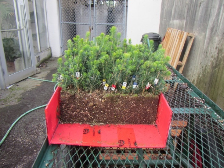
In our first experiments we studied interior lodgepole pine (Pinus contorta ssp. latifolia) populations. For this species, mean annual temperature (MAT) of the seed source is the variable revealing the strongest patterns of correlation with growth (Wang et al. 2006). ClimateWNA (Wang et al. 2012) data were used to plot the map of MAT below.

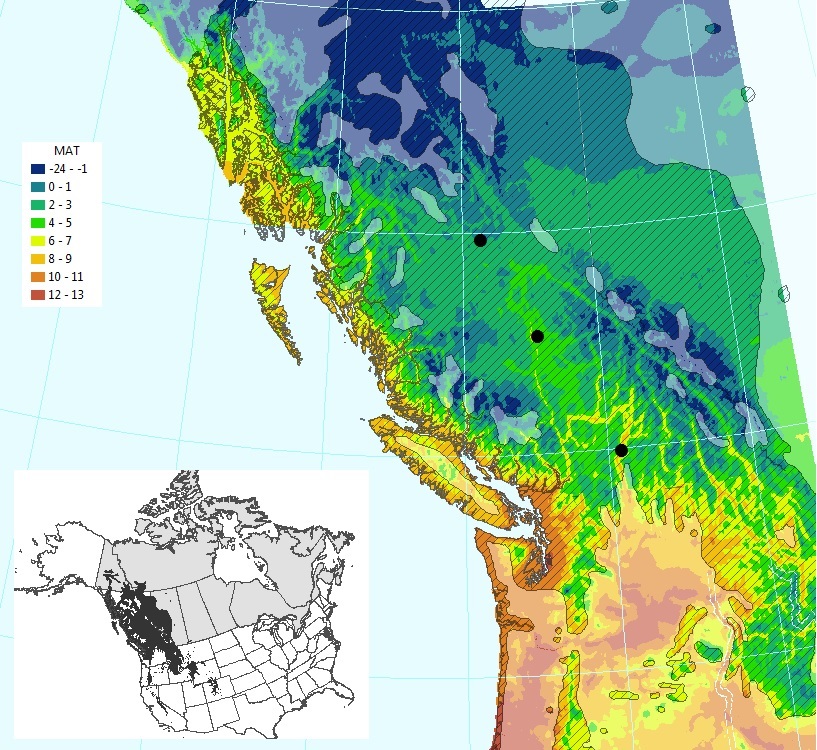
Natural range of Pinus contorta in North America (insert, dark grey) and detail of climate conditions (MAT, °C) in the area of interest (British Columbia, excluding the milky-white overlay where the species does not occur). Three chosen locations with representative climates (black dots).

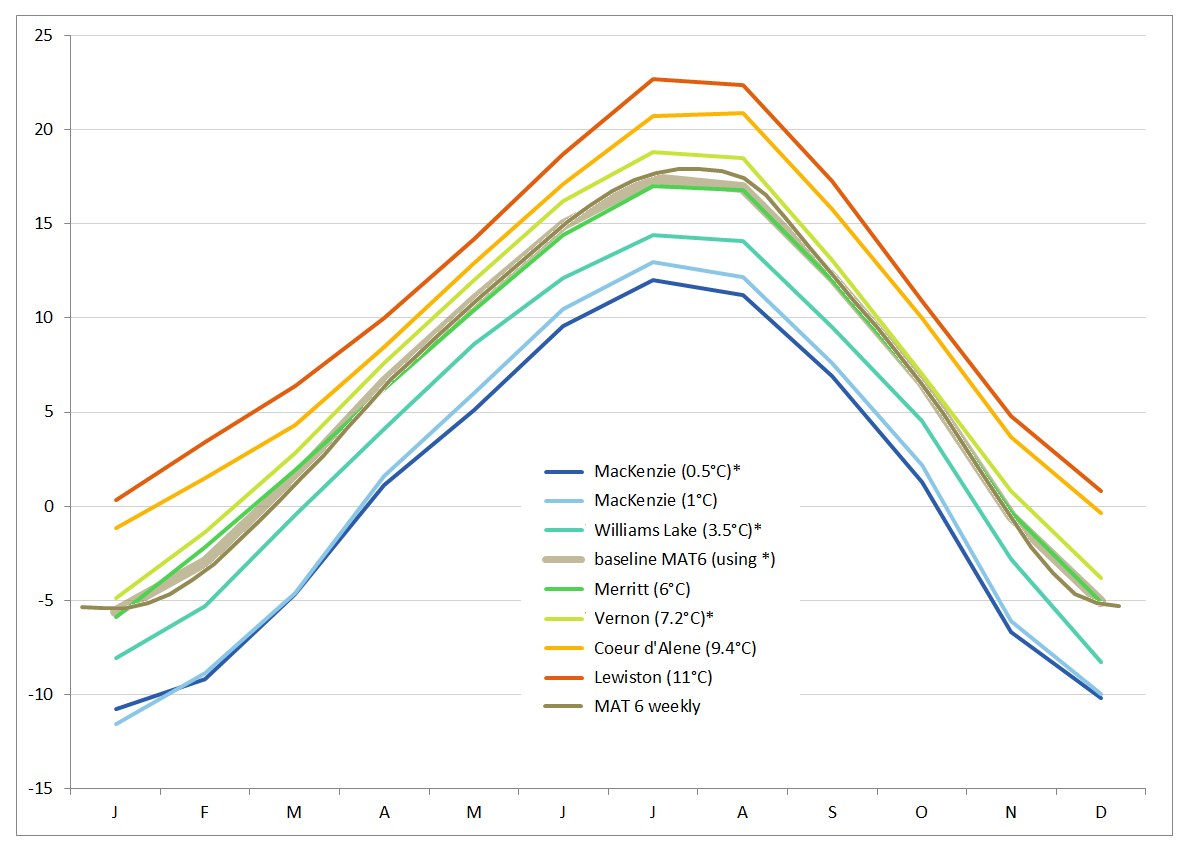
Our range of interest was interior British Columbia (BC), MAT 1 to 10 °C, to fully capture the growth response functions derived from field data (Wang et al. 2006). The geographic range for ssp. latifolia does not incorporate any areas with MAT 10°C, so this warmer, future climate regime was created by extrapolation. No attempt was made to average the climate for all the points with the same MAT. Instead, three points were chosen on the map, with MAT close to 1, 4 and 7°C, which had weather stations nearby. Such proximity is not really required, since ClimateWNA also provides detail on average daily ranges, but is still useful to inform us about the absolute maximum temperature. Other species may require other approaches, depending on the climate variables that best explain their adaptation. Now that a target climate has been chosen, find out how I developed realistic temperature regimes, moisture regimes, and where you can find suitable photoperiod data. Over the next several days, we’ll be posting on simulating winter conditions, heat waves, stimulating germination and bud set. At the end of the story, you will be familiar with most of the methods we had to use for growing plants for our AdapTree project. If you have tried similar or even stranger things, let me know. I’m curious to find out!