Okay so I came back and looked at the recommended BreachLeastCostDepressions tool from Whitebox. When I ran it previously I did not understand what “dist” was. For a full explanation by Dr. John Lindsay himself, check out this post.
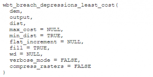
In summary, “dist” (as seen in the code above) is the “maximum search distance for breach paths in cells”. The tool “BreachLeastCostDepressions” basically analyses each pit cell then searches for the next lowest cell around it. The search radius grows until a lower cell is found and then they are connected and a breach channel is carved. By setting “dist”, you are effectively limiting how far this search radius will go. It is important to set this because if you do not, a breach channel between two low cells could be dug across significant ridges. However, quite often it resolves itself before jumping across ridges (i.e. it’s typically able to find a lower cell with a relatively short radius). A value of 10 and 100 both seemed to give me good results. Because this is a computationally demanding tool I also tried FillDepressions to speed things up. The results were as follows with the orignial .asc file on the left followed by BreachLeastCostDepressions (dist = 10), BreachLeastCostDepressions (dist = 100), and FillDepressions.
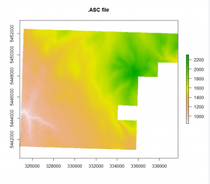
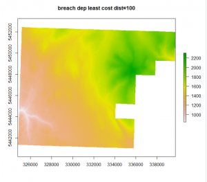
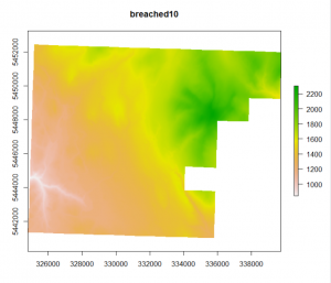
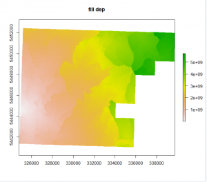
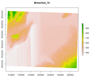
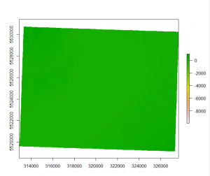
As you can see, the first three all look the same but FillDepressions seems to be changing things around more than I would like. Because breach least cost was taking so long I tried pre-processing with fill_single_cell_pits or breach_single_cell_pits to reduce the infilling required in one go but it still took too long. The other problem was that even after it ran, my resulting raster had weird lines in it and every time I infilled pits, it would fill in everything (see the raster to the right below). This was likely because it was picking out the natural undulations of my high-resolution DEM (1-m) and flagging them all as pits.
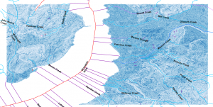
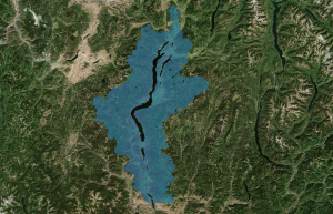
I decided to resample the whole thing to 10m (since I will be resampling everything to 10m anyways to match my multispectral sentinel data). By resampling my files to 10m, it allowed me to bypass the breaching step since there are not likely to be any artifacts or pits remaining. The resulting TWI looked WAY better and lined up nicely with the existing BC gov stream network:
Because this worked so well for one of my files, I then mosaiced all 84 files into one big raster and ran the following functions from Whitebox on the large raster:
~~~~~~~~~~~~~~~~~~~~~~~~~~~~~~~~~~~~~~~~~~~~~~~~~~~~~~~~~~~~~~~~~~~~~~~~~~~~~~~~~~~~~~~~~~~~~~~~
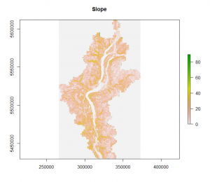
##FIRST run slope
wbt_slope( dem = “P:/AserLab/Projects/OK_Wetlands/Mega_Raster_10m/Mega_Raster.tif”, output = “P:/AserLab/Projects/OK_Wetlands/Slope/AllFiles_Slope_10m”, zfactor = NULL, units = “degrees”, wd = NULL, verbose_mode = FALSE, compress_rasters = FALSE ) slope <- raster(“P:/AserLab/Projects/OK_Wetlands/TWI_NEW/AllFiles_Slope_10m.tif”)
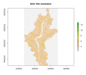
##NEXT run SCA – no pit filling req since artifacts were probably dealt w when I resampled to 10m.
#Run first w log=TRUE to visualize, then run w log=FALSE for final output
wbt_d_inf_flow_accumulation( input = “P:/AserLab/Projects/OK_Wetlands/Mega_Raster_10m/Mega_Raster.tif”, output = “P:/AserLab/Projects/OK_Wetlands/TWI_NEW/AllFiles_SCA_10m.tif”, out_type = “Specific Contributing Area”, threshold = NULL, log = FALSE, clip = FALSE, pntr = FALSE, wd = NULL, verbose_mode = FALSE, compress_rasters = FALSE ) flow <- raster(“P:/AserLab/Projects/OK_Wetlands/TWI_NEW/AllFiles_SCA_10m.tif”)
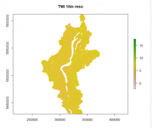
##NOW run Wetness index
wbt_wetness_index( sca = flow, slope = slope, output = “P:/AserLab/Projects/OK_Wetlands/TWI_NEW/AllFiles_TWI_10m.tif”, wd = NULL, verbose_mode = FALSE, compress_rasters = FALSE )
~~~~~~~~~~~~~~~~~~~~~~~~~~~~~~~~~~~~~~~~~~~~~~~~~~~~~~~~~~~~~~~~~~~~~~~~~~~~~~~~~~~~~~~~~~~~~~~~~
It worked well and was fast to process. The featured image at the top of my post is my resulting TWI visualized in QGIS.
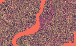
I wanted my TPI data to match at a 10-m resolution as well so I reran it on the large mosaicked raster with good results. I had to adjust for the 10-fold difference so rather than TPI100 and TPI750 I used TPI10 and TPI25. TPI10 is pictured below.
Things run smoothly once your data is in the right format and you know what you’re doing.
Leave a Reply