Topographic Wetness Index (TWI) – PART ONE

As a recap, I am currently making my way through a long list of parameters that I am interested in for mapping wetlands. These parameters are to be calculated from the raw lidar data (.laz files) or  from the Digital Elevation Model (DEM) data (.dem or .asc files) derived from the lidar. So far I have successfully run TPI (Topographic Position Index – see my last post). Next on the list is the Topographic Wetness Index (TWI).

What is TWI?

TWI is a commonly used index in hydrological analysis for describing the tendency of an area to accumulate water. It basically tells us how likely an area is to be wet. Important for wetland identification as you can imagine. It is based on slope and contributing area. Areas with higher topographic wetness index values are likely to be wetter relative to areas with lower values. The calculation is as follows, where SCA is the specific catchment area and φ is the slope angle. 

TWI=ln(SCA/tanφ)

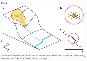
Figure from Mattivi et al. 2019.

Slope is easy enough to calculate from the DEM and a simple function can be run to do so (I ran all of my calculations through WhiteBox-GAT, more on that below). The calculation of SCA is a bit more complicated. Specific Catchment Area (SCA) is defined as the contributing area per unit width of contour  (i.e. the catchment area divided by the flow width). The contributing area (aka basin) represents the size of the upslope area draining into a cell. To calculate the contributing area, a flow routing algorithm is used. This quantifies how the water flows on the land surface and establishes the direction of the flow for every cell. There are a variety of algorithms that have been created for this purpose. They fall within two main categories: single flow direction and multi flow direction.

Deterministic eight-node (D8) is a common single flow direction algorithm by O’Callaghan and Mark, 1984 (see also Garbrecht and Martz 1997). It determines the flow direction based on the steepest descent toward one of the eight neighboring cells. The problem with this model is that it tends to concentrate along distinct, often artificially straight lines. Another problem occurs when the steepest gradient falls between two of the eight cardinal and diagonal directions (López-Vicente et al. 2014).  There are other algorithms which try to correct for these problems such as the quasi-random eight-node algorithm (Rho8), which introduces a degree of randomness to break up parallel flow paths (created by Fairfield and Leymarie, 1991) and results in more realistic-looking flow networks. There are downsides to this as well such as the randomization causes more cells to be without upslope connection and it is not replicable (i.e. each time the algorithm is run it produces a different flow pattern)  (López-Vicente et al. 2014). I could go on and on about flow accumulation models but I guarantee López-Vicente et al. (2014) will do a better job (see their algorithm comparison paper here). When deciding which algorithm to use, I decided to follow in the footsteps of Higginbottom et al. 2018. These researches used a topographic wetness index for mapping wetlands and determined flow direction using the D8 model.

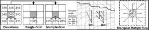
Figure from López-Vicente et al. (2014).

There are many different software options for computing TWI. Mattivi et al. 2019 provide a good comparison between different open source GIS platforms for calculating TWI if you are considering running TWI yourself, see their paper here. I attempted to use SAGA-GIS for this purpose; however, it did not like the format (or maybe it was the size) of my files (I have 84 ascii files ~1.25GB each). I decided instead to use WhiteBox-GAT again (I used this also to calculate TPI). There are a variety of flow accumulation model options available by John Lindsay and the WhiteBox Tools User Manual can be found here.

The D8FlowAccumulation model requires the input DEM to be hydrologically corrected to remove depressions and flat areas. It is recommended that this is achieved using the BreachDepressionsLeastCost or FillDepressions tools. I tried to run BreachDepressionsLeastCost; however, it was computationally demanding and I couldn’t get my output to look right so I ended up just running BreachSingleCellPits (a pit is a single DEM cell that is lower than all of its neighbours). The costs and benefits of different depression filling techniques are further explained by Lindsay 2016. There is also good info in this article by ESRI.

Figure from: arc-gis blog written by Caitlin Scopel “Optimized Tool for DEM Pit Removal Now Available“.

 I think I need to come back to this and ensure that BreachSingleCellPits was the appropriate course of action here.  Once the pits were breached, I ran the D8 model on the breach-filled DEM to get SCA. I ran a slope calculation on my DEM then fed both outputs into the TWI calculation. The one thing I did not double check was what the impact of analyzing one tile at a time might be for a flow accumulation model. The concern here is if the tile does not capture the entire catchment area or basin then flow input sources might be missed. I will need to look into this further as well.