Topographic Position Index (TPI)

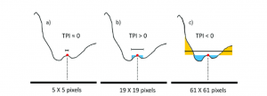
What is TPI? The topographic position index helps us distinguish topographic features such as a hilltop, valley bottom, exposed ridge, flat plain, upper or lower slope. It is calculated by comparing the elevation of each pixel to its surrounding neighbours. The number of neighbours you compare it to (i.e. the size of the neighbourhood) makes a big difference (i.e. 5×5, vs 19×19 vs 61×61). See graphic below (additional info here).

TPI = zero/near-zero – flat or a near continuous slope.

TPI = large positive – the central pixel is much higher than the surrounding areas; ridge or hill.

TPI = large negative – the central pixel is much lower than the surrounding areas; bottom of a valley or gulley.

M. A. Salinas-Melgoza, M. Skutsch, and J. C. Lovett (2018): Predicting aboveground forest biomass with topographic variables in human-impacted tropical dry forest Ecosphere 9(1):e02063. 10.1002/ecs2.2063

Quick pause, to define some terms: “neighbourhood size” “pixel size” “radius” “scale” and “moving window”. Neighbourhood size is the generic term meaning “the size of the area around each pixel that we are looking at” and can be represented by the number of pixels, or (given that we know each pixel = 1 square meter) by meters. That is, a radii of 1, 2, 3… yields a square filters of dimension 3 x 3, 5 x 5, 7 x 7… which is an area of 9, 25 and 49 square meters (in my case because each pixel = 1 square meter). You can also have a circle radius if your focal point is a point rather than a pixel. “Scale” means the size of the moving window used to calculate the index. “Moving window” is the same as neighbourhood, which again defines the vicinity used to calculate the mean value to which values from individual cells are compared.

The selection of an appropriate neighbourhood size is crucial in the calculation of the TPI. Calibration to field condition must be done by the researcher based on the individual site characteristics using trial-and-error. Smaller neighbourhood sizes are better at picking up small-scale features and larger neighbourhood sizes are better at picking up large features. The optimal neighbourhood size will depend on what you’re interested in viewing as well as what the natural landscape is doing (is it flat? mountainous? homogenous? heterogenous?).

Here are some other papers that have used varying neighbourhood sizes for the calculation of TPI:

• Weiss 2001 utilizes both a small and large scale TPI to characterize the landscape near Hood, Oregon. The scale of 300m reflects the degree that the stream channel is incised and the narrowness of the valley. The scale of 2000m reflects the broader valley morphology and the relative relief of streams and their surrounding topography.
• DeLancey et al. 2019 used a 500 m moving window to calculate TPI in the boreal peatlands of Alberta, Canada.
• Zwolinski & Stefańska (2015) were characterizing an alpine area and a river drainage basin. For the drainage basin, a window of 7 × 7 cells (217 × 217 m) proved the most suitable. Whereas for the mountains, a window of 9 × 9 cells (90 × 90 m) was the best. They concluded that the more diverse the relief of the area under study, the smaller calculation window should be used.
• Deumlich, Schmidt and Sommer (2010) conducted a terrain analysis in NE Germany using neighborhood sizes of 25 m and 500 m for small and large landform elements, respectively. The determination classes and neighborhood sizes were chosen to optimize and to represent the typical landforms of the region (short and large slope length of different inclination, the occurrence of hummocks and holes).
• Liu et al 2010 utilized both 5×5 and 10×10 grids (each cell =250 x 250m) for TPI in their analysis of terrain in the Great Xing’an Mountains, NE China.

Consistent in most of these studies is that they use different scales of TPI analysis – one with a small neighbourhood to catch the small-scale features and one with a large neighbourhood to catch the large-scale features. By combining the parameters from two neighbourhood sizes, it allows us to identify complex landscape features and provide more information about topography (Weiss 2001). Given that the landscape around Kelowna is mountainous with flat valley bottoms (and is therefore quite heterogenous), I will be calculating two scales of TPI.

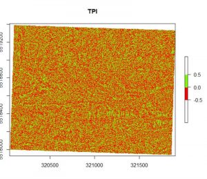
Software and methodology for calculating TPI: When I first ran TPI, I used the gdaldem function from GDAL in R, which by default (and you’re not able to change this) uses a very small neighbourhood. It is calculated by subtracting the mean elevation of the 8 surrounding cells from the central location’s elevation (1-pixel radius = a central points 8 immediate neighbours). This is only good for identifying fine scale features. This worked for some of my files but other files ended up looking like speckled nonsense where there should have been rivers and valleys. I need to run a bigger neighbourhood size.

Instead of gdaldem, I will use WhiteBox-GAT, through the R-interface (I’ve been really enjoying the versatility of this program, THANK YOU JOHN LINDSAY). From the studies mentioned above, I might be looking in the realm of 100 to 2000-m for my neighbourhood size, and I already know I want to calculate both a small scale and large scale TPI in my list of parameters. From what I can tell, Topographic Position Index is synonymous with Difference From Mean Elevation, which is an absolute Local Topographic Position Index (Newman, Lindsay, Cockburn 2018; Wilson and Gallant 2000; Deumlich, Schmidt and Sommer 2010). The WhiteBox-GAT does not list “TPI” in its tools. Instead, it uses “DiffFromMeanElev” (see WhiteBox Tools Library for more info):

DiffFromMeanElev: This tool can be used to calculate the difference between the elevation of each grid cell and the mean elevation of the centering local neighbourhood. This is similar to what a high-pass filter calculates for imagery data, but is intended to work with DEM data instead. This attribute measures the relative topographic position.

wbt_diff_from_mean_elev(
dem,
output,
filterx = 11,
filtery = 11,
wd = NULL,
verbose_mode = FALSE,
compress_rasters = FALSE
)

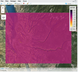
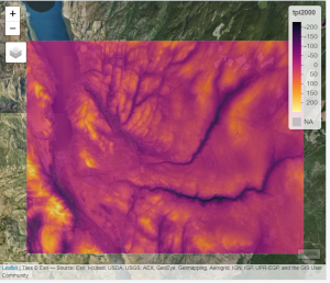
After trial and error, the following neighbourhood sizes (tpi100 & tpi 2000) seem to be sufficient for my purposes (viewed using Leaflet in R):

References:

Deumlich, D., Schmidt, R., & Sommer, M. (2010). A multiscale soil–landform relationship in the glacial-drift area based on digital terrain analysis and soil attributes. Journal of Plant Nutrition and Soil Science, 173(6), 843–851. https://doi.org/10.1002/jpln.200900094.

Lindsay JB. 2016. Whitebox GAT: A case study in geomorphometric analysis. Computers & Geosciences, 95: 75-84. DOI: 10.1016/j.cageo.2016.07.003.

Liu, H., Bu, R., Liu, J., Leng, W., Hu, Y., Yang, L., & Liu, H. (2011). Predicting the wetland distributions under climate warming in the Great Xing’an Mountains, northeastern China. Ecological Research, 26(3), 605–613. http://dx.doi.org/10.1007/s11284-011-0819-2.

References:

DeLancey, E. R., Kariyeva, J., Bried, J. T., & Hird, J. N. (2019). Large-scale probabilistic identification of boreal peatlands using Google Earth Engine, open-access satellite data, and machine learning. PLoS One, 14(6), e0218165. http://dx.doi.org/10.1371/journal.pone.0218165.