In my last post I briefly mentioned a few broad datasets I will be using: Multispectral data, radar, and LiDAR.
I will begin my quest to making a predictive wetland map by digging into the LiDAR data since it will require the most processing. There have been numerous studies that have used LiDAR for mapping wetlands, each of which indicated a list of useful parameters that they used to make their models. Things like DEM, CHM, TPI, TWI, grid statistics, LAI, LSI, AGB… so. many. acronyms. I compiled a list of my own which includes the most important and widely used parameters. I will attempt to calculate these for my own model.
Before diving into what some of these acronyms mean, I should first explain how the LiDAR data is actually saved and what it entails. The LiDAR data was collected by the Ministry of Forests, Lands, and Natural Resource Operations and Rural Development, BC following the provincial specifications for airborne LiDAR (v 3.0). More or less, a plane was flown at 1000-m above ground over the Okanagan and shot laser beams down toward the earth as it went (harmless lasers). Each time the laser bounced off something, it returned to the sensor and one point was logged. The target density was set to 30 points per square meter. Some of these laser beams bounced off the tops of trees, the middle of the trees, off buildings, off shrubs and some even penetrated through the vegetation and bounced off the ground. If you have a close look at the image below, you will notice that the landscape is a ravine with trees in it and if you look really closely, you will see the individual points/laser returns. This is called the “3D point cloud”.
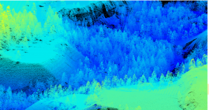
The 3D point cloud is pretty to look at but in order to analyze it, summarize it, characterize it… we need to turn these points into values – we need numbers. Given that there are so many points, we have many options as to how we can summarize this data. Each point has associated with it an x, y, and z value (lat, long and elevation). In order to turn this 3D point cloud into a 2D raster with numbers, we need to overlay a grid and summarize all the points that land in each square (or pixel).

This photo was taken from Selvam et al.’s (2019) intro to GIS paper (I highly recommend checking it out here).
What values do we actually care about for mapping wetlands? Well to start, it’s important to know what the ground looks like so we can predict where water might pool. It makes sense that the ground would be the lowest returned points in a given area (i.e. having the lowest z-values), so we save all those points and scrap the rest. This is called the Digital Elevation Model (DEM).

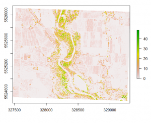
We know vegetation is important for mapping wetlands and from our 3D point cloud we can isolate just the vegetation and later define it as grass, trees, shrubs, etc. This is the Canopy Height Model (CHM).
What I haven’t mentioned is that along with an x, y, and z value, each of the points from the point cloud also has an intensity value (i), which gives us information about how strongly the return bounced back… if you can imagine shining a light beam at a hard, reflective surface, the light will be returned to you brightly, compared to a rugged surface or vegetation where it might come back much dimmer… intensity is good for indicating areas where there is standing water.
As you can imagine, there are countless ways to summarize this data. Millard & Richardson (2013) investigated over 100 variables when mapping bogs in Southeastern Ontario and reported eight of them to be particularly important. These final eight variables were a mixture of LiDAR DEM, DSM and discrete return derivatives, and morphometric terrain derivatives. Ultimately, the standard deviation of all laser returns and the residual of the DEM above/below a polynomial surface provided the greatest explanation of the variance between classes.
References:
Millard, K., & Richardson, M. (2013). Wetland mapping with LiDAR derivatives, SAR polarimetric decompositions, and LiDAR–SAR fusion using a random forest classifier. Canadian Journal of Remote Sensing, 39(4), 290–307.
Leave a Reply