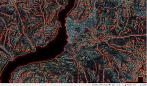
MTP is an image output that allows the viewer to visualize a landscape using various scales of topographic position. By utilizing a local-, meso-, and broad-scale topographic position, prominent features at each scale can be visualized at once (Lindsay et al 2015). Inputs are calculated from the maximum deviation from mean elevation (DEVmax) function in Whitebox (Lindsay et al. 2015). The MTP output display these varying scales in blue (features prominent at the local-scale), green (features prominent at the meso-scale), and red (features prominent at the broad-scale). Other colours occur when a feature is prominent across multiple scale ranges.
Previously I had calculated TPI using the DiffFromMeanElevation tool at different scales by adjusting the neighbourhood size. This measures relative topographic position by calculating the difference between the neighbourhood or window’s center elevation and its mean elevation (Lindsay 2015; Wilson and Gallant, 2000; Weiss, 2001). It has the same units as elevation and is either positive, indicating an elevated location, or negative, indicating a low-lying position. Unlike the DiffFromMeanElevation, DEVmax is a unitless measure of relative topographic position that is scaled by the local ruggedness. It is calculated in the same way as the DiffFromMeanElevation except that the elevation difference is normalized by the standard deviation of elevation. This characteristic is particularly useful in applications involving heterogeneous landscapes (De Reu et al. 2013; Lindsay 2015).
To calculate MTP, I used the Whitebox plug in in QGIS. The scale parameters are in units of grid cells and specify kernel size “radii” (r), such that: d = 2r + 1. That is, a radii of 1, 2, 3… yields a square filters of dimension (d) 3 x 3, 5 x 5, 7 x 7. I played around with different values of r and landed on the following:
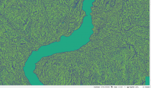
Local scale (r = 3-5): 3 = 7×7 = 70 x 70 m // 5 = 11 x 11 = 110m x 110m
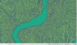
Mesoscale (r = 5-10): 110m – 210m
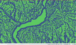
Broadscale (r = 20-50): 410m – 1,010m
Previously, I had used the following DiffFromMeanElevation values in my model:
TPI1, = 3×3 window size = 30m x 30m for my data.
TPI20 = 41 x 41 = 410m x 410 m
*it would be interesting to study the effects of small vs large neighbourhood sizes for identification of wetlands.
The resulting MTP looked like this:
References:
Lindsay J, Cockburn J, Russell H. 2015. An integral image approach to performing multi-scale topographic position analysis. Geomorphology, 245: 51-61.
Leave a Reply