Recently I ran into a stone wall when I tried to analyse the time series data from my first-year experiments.

In my experiments, I measured tree sap flow velocity and different environmental controls such as temperature, solar radiation, relative humidity, wind speed and soil moisture. However, these data were at different time steps. The sap flow velocity were at a hourly basis, while the environmental controls were measured at either every 10 minutes or 20 minutes. So I had to aggregate those into the same time sequences.

There are two types of aggregating data. The first is to assemble these data at every hour at each date, in order to make a correlation analysis or multiple linear regression; and the second is to average data which are measured at the same hour, disregarding the date, aiming at analyzing the 24-hour profile of the variables.

Thanks to R, I succeeded in dealing with my four-month data at just ten seconds. Now, I’d like to share the codes with you, giving my soil moisture data as an example.  🙂

1. Making a 24-hour profile of soil moisture

Here is part of my soil moisture data (unit: VW%) at my Treatment 2 plot. I measured the soil moisture at two depth: Shallow ( at the 20 cm depth), and Deep (at the 40 cm depth).

Fig. 1 Example of initial soil moisture data

(1) Save the excel file as *.csv, and import it into R Studio. In my case, I input my data as data frame named soilt2. Please remember to change the data type of Datetime column as Datetime, and turn Shallow column and Deep colunm as numeric.

Fig. 2 Input soil moisture dataset

(2) Input code:

soilt2$Datetime1 <- as.POSIXlt(soilt2$Datetime)$hour  ### This will add a new colunm named Datetime1 in the soilt2 dataset. Datetime1 displayed below showed that only the hour was extracted from Datetime.

Fig. 3 the added new colunm Datetime1 is showed on the right of the table.

soilt2 <- aggregate(cbind(Shallow, Deep) ~ Datetime1, data=soilt2, FUN=mean) ### This averaged Shallow and Deep data into hourly data,  regardless of the date. In my case, I changed my original dataset. If you don’t want to make change of the original dataset, please give a new name to your new dataset, such as soilt3.

Fig. 4 The changed soilt2 data frame.

Done! Yay!

2. Assemble the data at each hour at each date.

(1) Import the dataset (the same as the first method).

(2) Input the following code

soilt2$Datetime2 <- droplevels(cut(soilt2$Datetime, breaks=”hour”)) ### This added a new colunm named Datetime2 in soilt2, which includes the date and the hour extracted from Datetime column.

Fig. 5 The added new column Datetime2 is showed on the right of the table.

soilt3 <- aggregate(cbind(Shallow, Deep) ~ Datetime2, data=soilt2, FUN=mean) ### This calculate the mean of data in each hour at each date.

Fig. 6 The new soilt3 data frame.

Yay again! Done!

If you want to output these data into excel, you can load package (xlsx), and using the code of write.xlsx(  ).  For example, I use the following code:

write.xlsx(soilc1, “c:/Users/Yi Wang/Desktop/soilc1.xlsx”)

There are definitely other ways to aggregate the data, but the codes that I put on this blog, in my opinion, is the most simple code. If you disagree with me, or you’d like to share your code, please feel free to leave your comments.

Thank you for reading!

May, 04, 2017

Have you ever experienced a problem that R failed in recognizing part of your time series data, and analysed them by omitting thousands of rows in your spreadsheet?

You then looked for the cause, and found that the time format of your data seemed to have subtle inconsistency in Excel. Some parts of the time data were Text-type (e.g., from row 335 to 344 in Fig. 1), while the other parts were Datetime-type (e.g., from row 324 to 334 in Fig. 1), though these data were downloaded from the same data logger at the same time.

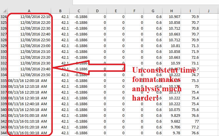
Fig. 1 A screenshot of my data, illustrating the inconsistency time format problem.

So you tried to make the time format consistent, by selecting the whole column (e.g., Column A in Fig. 1), right-clicking, entering the Format Cells box, and choosing the desired format (e.g, in my case, I chose custom format, mm/dd/yyyy h:mm).

However, you found that this didn’t work on your Text-type data. So you tried again, and unfortunately, failed again. You even tried different types of paste and copy, but had no effect. After tens of failures, you gave up and decided to manually re-type time data row by row into the spreadsheet to amend the format, but “millions” of Text-type data which embellished in your good Datetime-type data here and there drove you crazy. You started to worry that you would be stuck in typing data for the rest of your life.

What’s worse, the Datetime-type data were also problematic, because Excel recognized months as days, (e.g., in Row 334 in Fig. 1, 12 is actually the day). You could also not be able to correct them by just changing the format setting. What a pissed-off moment!

Fig. 2 Only Rage Face can express my "rage" on Excel. Hahahaha....

But don’t be frustrated! I had fought with this moment many times, and eventually defeated it. Now, I’d love to share my tips with you on how to deal with this problem.

Why did this problem happened?

I have searched for the cause for a long time, and found that people who claimed the similar problems are most in Canada. So I speculated that the problem came from system regional setting. Later, I found other peoples’ explanations on the causation, which confirmed my speculation.

According to their explanations, if you imported US format (mm/dd/yyyy) time series data from your data logger into your computer which set as Canadian English/French format (dd/mm/yyyy), then Excel would mistake days as months when the days are under 12, while leave the rest (the days are greater than 12) as unrecognized, text-type data.

Here are two discussions I found on Stack overflow (http://stackoverflow.com/questions/4660906/some-dates-recognized-as-dates-some-dates-not-recognized-why)

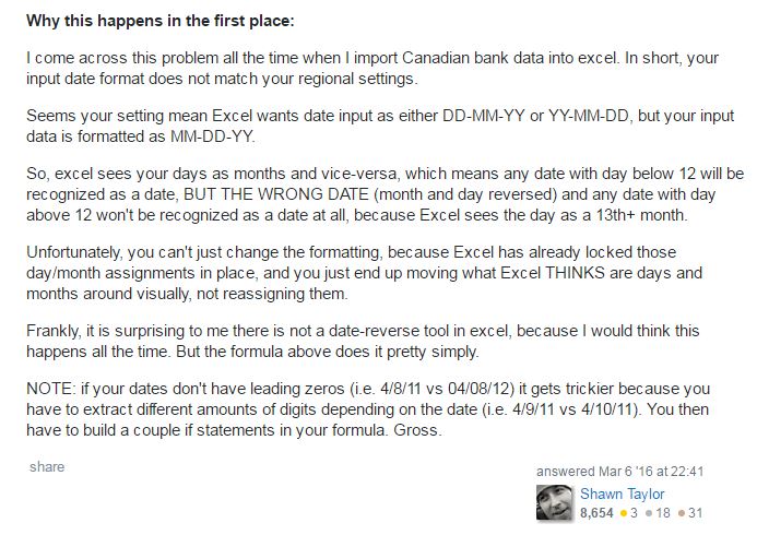
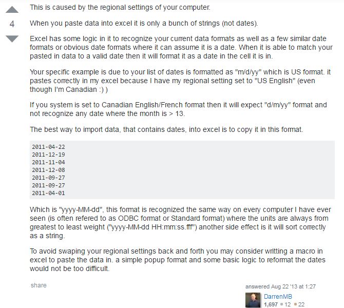
Fig. 3 Other peoples' discussion on the same issue at Stack Overflow.

How to deal with this problem?

Firstly, check date settings in your computer.  

Click the time display at the right bottom of desktop to enter the Date and Time box, and click Change date and time…, entering Date and Time setting, and then click Change Calendar Setting, entering Region and Language box. Under Format tab, you can modify time format under Short date and Long date. In my case, I prefer MM/dd/yyyy to dd/MM/yyyy as the short date format in my computer.

This step helps you to avoid any further problem, if you need to import your data from external sources such as your data logger.

Fig. 4 Time format setting in the Window system.

Secondly, modify the wrong Datetime-type data.

(1) Change your wrong Datetime-type data into Text type data, by using TEXT Function. For example, the data in Column A, Row 329 is 12/08/2016 11:00:00 PM, with a custom format of mm/dd/yyyy. I use function: =TEXT(A329, “dd/mm/yyyy H:MM”) to convert it into Text-type data. Please note that I use format “dd/mm/yyyy” instead of “mm/dd/yyyy”, in order to exchange “months” with “days”.

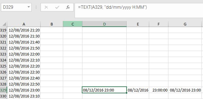
Fig. 5 My illustration on how to convert Datetime-type data into Text-type data.

(2) Convert Text-type data into Date-type and Time-type data,by using DATE Function and TIME function. I used =DATE(MID(D329,7,4), LEFT(D329,2), MID(D329,4,2)) and =TIME(MID(D329,12,2),MID(A337,14,2),0) in Cell (E, 329) and Cell (F, 329) separately. Please note that in my case, I don’t need seconds, so I put 0 in the time function. Then I gathered Date and Time together at Cell (G, 329) by simple addition: E329+F329. You can also complete those steps at one time by putting DATE and TIME functions together in one cell. 

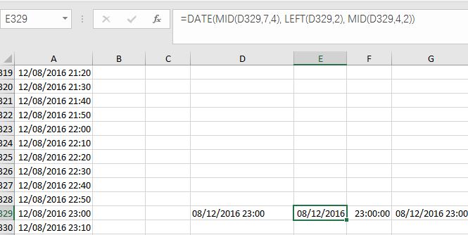
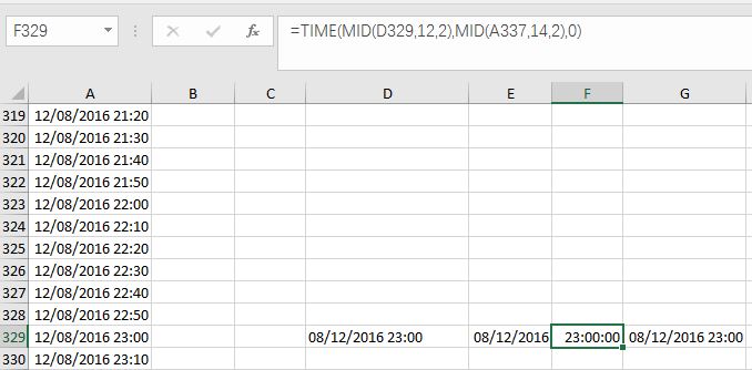
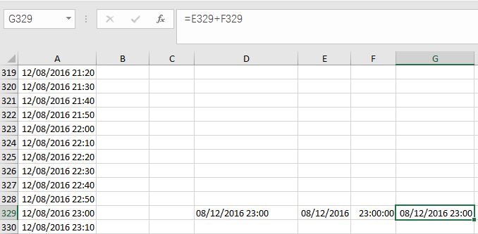
Fig. 6 My illustration on how to convert Text-type data into Datetime-type data.

Here is a detailed introduction on TEXT, DATE and TIME Functions:

                    Format                                                 Example

TEXT (Cell, “desired format”)   ==> TEXT(A329, “dd/mm/yyyy H:MM”)

DATE (year, month, day)           ==> DATE(MID(D329,7,4), LEFT(D329,2),MID(D329,4,2))

TIME (hour, minute, second)    ==> TIME(MID(D329,12,2),MID(A337,14,2),0)

In addition, here are the how the extract functions like MID and LEFT work:

MID (Cell, The location of first character to extract, the number of extracted characters)

MID Function extracts characters from inside of the string. For example, MID(D329,7,4) is equal to “2016”, because the “2” of “2016” in Cell D329 is the 7th characters, and 2016 consist of four characters.

LEFT (Cell, the number of extracted characters)

LEFT Function extracts characters starting from the left of the string. For example, LEFT(D329, 2) is equal to “08”, because “08” are first two characters at the left.

Please note that space or symbols like “/”, “:” or one space “”, are counted as one character.

Thirdly, convert other Text-type data into Datetime-type data by using the same functions introduced above.

You may encounter a new problem when your Text-type data contains “am” or “pm”. Unfortunately, I didn’t find a function to extract “am” or “pm” into 24-hour system. But you can use subtraction to overcome this problem.

For instance, Cell D337 is “08/13/16 12:10:18 AM”. If I use TIME(MID(A337,10,2),MID(A337,13,2),MID(A337,16,2)), then Excel gives me the result as “12:10:18” in the 24-hour system, which is “12:10:18 pm”.

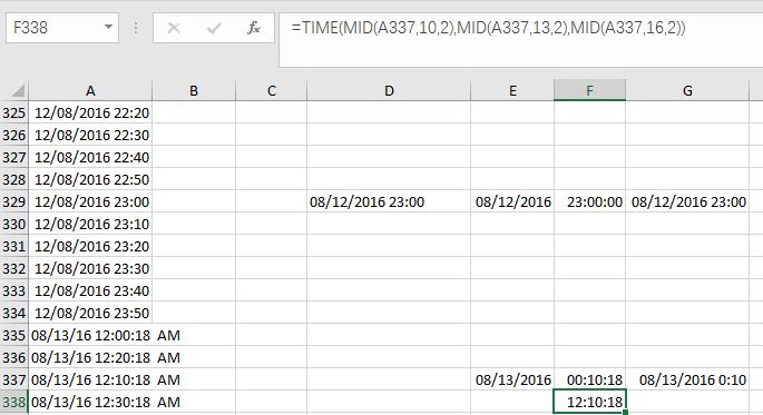
Fig. 7 Illustration on how to deal with "am" or "pm" in your data.

So instead, I used TIME(MID(A337,10,2) -12,MID(A337,13,2),MID(A337,16,2)), and Excel gave me the exact result that I want, the “00:10:18”.

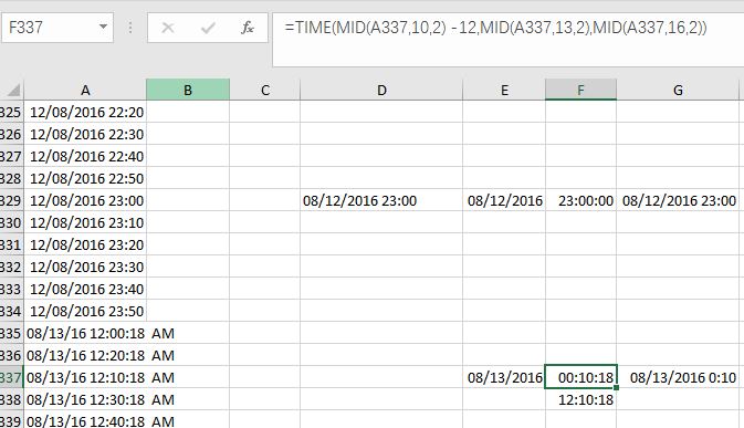
Fig. 8 Illustration on correct your time data by simple subtraction.

With above three steps, you can successfully arrange your “naughty” time series data in the “stupid” Excel. Life turns beautiful again!

If you have know more convenient ways to deal with this problem, please tell me by leaving your comments here. 🙂

Thank you for reading it!

April, 28, 2017

With the lesson drawn from last field trip, we chose a normal day to the field. It was not warm nor too cold. Adam, Antonio and I went to the field to finish measuring DBH. Since the color spray didn’t work well, we brought ties and staples to mark the position. We wrapped the  orange tie around the trunk at the breast height, and fixed it with staples. The staples should be in the middle of the caliper next time when we measure DBH again. Antonio marked the trees, while Adam and I measured and record the data. We even re-measured the Block 3.

At around 2:30 pm, everything was done! This is the end of experiments this year. Yay!

It is the end of October. Everything was covered by snows. It might be the last time of our field trip. we took some important equipment back last time, but we haven’t measured tree DBH yet. This data are very important, because it should be regarded as the end of the growing season in 2016, and the beginning condition of growing season in 2017.

In order to measure DBH, Antonio and I chose a sunny and warm day to go to the field. The sky was blue, and sun came up brightly in such a winter time. We thought that it would be a light work for us to measure DBH in such a beautiful day. However, things did go as easy as what we expected……

Because it was warmer, snows on the branches were melting and dripping down. We all soaked as we walked through the trees, which made the situation worse, because we felt colder and heavier! Later, our shoes became wet as well. We couldn’t move fast and steady. The ground was slippery. Sometime we fell off.

The snow melting no only made us feel freezed, but also damaged the electronic caliper for measuring DBH. We often stopped and used our clothes to dried it up when its readings stared to be unstable, though there were not actually dry clothes on us. We used our sleeves to dry caliper at the beginning, and the lower hem later, and then everywhere that was drier.

Our color spray didn’t work well, too. Pigments just joined in the drippings of melting and flowed down along the trunk, which made the trunks look like crying with colorful tears. We used the color spray, because we tried to reduce as many errors as we can, by marking the position that we measured on trees, since tree didn’t expand too much in a month. Next time we will measure DBH at the same position. We did not plan to use ties, because it restricted trunk’s expansion.

Anyway, as persistent person, Antonio and I insisted in staying there to finish our job. When We finished Block 3, I could not feel my feet anymore. I was really scared and exhaust. Antonio felt the same way. So we decided to stop measuring and come back at the other day.

Shaking with cold and disheartenment, we got into the car and drove back to Kelowna.

The site has already been covered by snow, but the car could still drive there, with cautions. We are approaching the end of experiment this year.

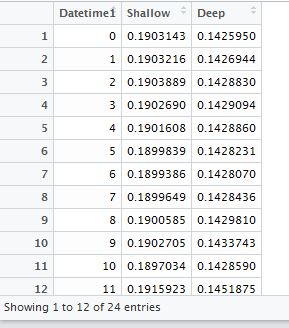
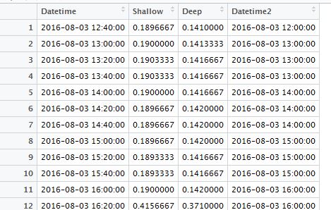
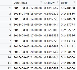
         Fig. 1 The road to my experiment site was covered by snow

In the winter, the temperature was assumed to below – 20 ℃. Some equipment like band dendrometer sensors and datalogger could be damaged by that freezing temperature. Thus, we decided to take them back.

               Fig. 2 Photo of B1T1 took at Oct, 18, 2016

Antonio and Guang went to the field with me on October, 18, 2016. We cut the wires of band dendrometer, and collected sensors into bags. Next year, we will use junction boxes and wire connectors to reconnect them.

Fig. 3 the band dendrometer sensors were taken back, leaving metal clamp and spring on the site.

We also unintalled the datalogger. It was not easy, as there were too many wires. Thanks to Antonio, we disconnected the wires without mixing them too much. Those wires were all marked with A, B, C, D …etc. So connection in the next year should be much easier. By the way, we disconnected solar panel and took the batteries back as well.  We protected the wires by tying and covering them with plastic films.

Fig. 4 the datalogger were taken back, and the wires were protected by plastic films

But sap flow probes were left on site, as suggested by a Dynamax consultant. Soil moisture sensors also stayed there. Climate stations will work through the whole winter. Hope that the memory of climate station is huge enough to store climate data of the whole winter.

Adam, Guang and I went to the field this time. We measured photosynthesis and stomatal conductance again. This time, the photosynthesis measured at the morning was almost the same with that measured at the afternoon. Weird! Anyway, I will measure more data in the future!

Last time, I felt that it was too tired to raise leave chamber all the time. As a handywoman, I decided to make some small “device” to freedom my arms. So I went to Value Village, a second hand store near where I live, to buy a small basket which was made of wood. Then, I brought it with two hangers (hanger was Antonio’s idea) to my lab. Antonio and I used wires, hangers, basket and bandage to make a leaf chamber holder which could hang on the branch. I also put some foams inside the basket to prevent chamber from damage. We were excited to see how it works.

Three “A”s went to the field this time (Adam, Antonio and Abby (me)) hhhh 🙂 However, the weather wasn’t good.  The rain came down when the machine was ready. So we had to go back, because this system was not supposed to use during the rain. High humidity not only affected measurement, but also destroyed the machine. But anyway, we were happy to see that the leaf chamber holder worked well.

I affirmed that the dead batteries in last field trip resulted from a wrong way of charging. This time, I was quite sure that the batteries were fully charged.

Antonio, Guang, John and I went to the field at 8:00 am on September, 14, 2016. Guang helped me to measure photosynthesis and stomatal conductance. We measured two variables on the same branch which we selected on August, 26. We succeed in establishing two light responsive curves by using auto-measuring program setting light intensity at 2000, 1500, 1000, 500, 250, 126, 60, 30, 15, 1 umol/m2s. Photosynthesis rate responded to light intensity gradient very well, but stomatal conductance showed less responsive. When I took data from last field trip together, the patterns were divergent. The stomatal conductance on August, 26 was not stable, which may due to the power failure of the system.

   

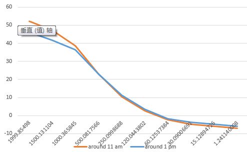
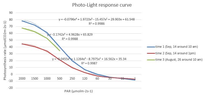
           Fig. 1 Light-responsive curves of photosynthesis rate

        

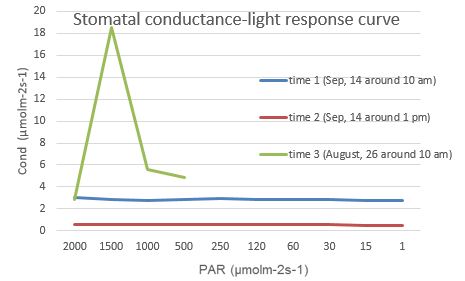
        Fig. 2 Light-responsive curves of stomatal conductance

We also measured photosynthesis rate under different temperatures in considering that temperature played an important role in regulating sap flow rate. But when we made the second temperature responsive curve, the batteries ran out. Actually, the temperature responsive curves didn’t seem good, because LICOR 6400 XT can not really control block temperature to higher or lower 3℃ than the ambient temperature.

          

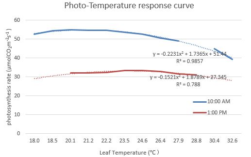
       Fig. 3 Temperature response curves of photosynthesis rate

        

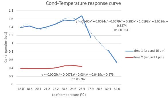
         Fig. 4 Temperature response curves of stomatal conductance

Photosynthesis rate and stomatal conductance varied at morning and afternoon, even under similar temperature and light intensity, with those in the morning were systematically higher than those in the afternoon.

After batteries ran out, we disassembled the machine, and then I downloaded data from datalogger.

Antonio and John helped me measure the tree height and DBH in all three blocks. However, I thought that it was not necessary to measure tree height in each month, because we used a four-meter ruler which was quite heavy and inconvenient to carry through forests. The most important reason was that this simple but crude measurement gave too many errors, as a majority of trees were around four meter, and did not have a significant increase in height in each month. I compared the tree height of previous month, and found that some heights in one or two month later were even lower than their previous values. I would discussed with Adam and Antonio about it.

Then, with the help of Antonio, I reconnected the wires of soil moisture sensors and put them in junction boxes. Some soil moisture sensors in T2 did not work well, which may be due to bad contact with soil, so we watered it and waited for the signals. Fortunately, the sensors started to report reasonable values. Antonio was genius!!!

We had achieved our goals today! 🙂

The main was to try LICOR 6400 XT to measure photosynthesis and stomatal conductance in this field trip. Before going to the field, I read the manual book, and replaced opaque conifer chamber with broad-leave chamber at my lab by myself. It was not easy, but I was really a handywoman.  hhhhh~  :‑D

              Fig. 1 I assembled opaque connifer chamber

I fully tested this machine with new chamber at my lab, with a cut branch of Ponderosa pine from the university campus. The machine worked well, so I decided to test it in the field.

At August, 26, 2016, Adam, Antonio, Guang and I went to the field. Adam assisted me by carry it, while Antonio and Guang checked the condition of other equipment at other plots.

Adam and I chose a east-faced, healthy branch of the tree in front of climate station at the T2 plot in Block 1 at 1.7 m height. There were some sparse branches below it, but seemed to be not very healthy. According to data from climate stations in three plots, the most significant difference of environmental variables in three plots was the solar radiation. So I hypothesized that differences in solar radiation contributed the most to contrast sap flow rates among three plots. Besides, I wanted to establish a model giving photosynthesis rate and stomatal conductance under different light intensities, in case there would be not enough field measurement data. Therefore, I measure light-response curve of branches as a preliminary experiment to see how photosynthesis and stomatal conductance response to light.

However, the battery of 6400 died soon, only after I measured four needle clusters (around 20 minutes). Adam was so worried about it, and told to me that if the problem came from the battery or machine, then we’d better send back them to the maintenance department as soon as possible.  But I felt embarrassed somehow, because I realized that I might not charge battery in a correct way, as the charger required to choose correct voltage and pressed fitted fuse into it, otherwise it always showed that battery was fully charged. I followed the guidebook carefully, but it still might be wrong.

I told to Adam about my speculation and sorry, and promised to him that I would check the problem and fix it as soon as possible. Adam gave his understanding, and suggested me to contact with Dr. Duan. Since batteries were dead, we disassembled the 6400 and put it back to the case.

Antonio and Guang also finished their works of checking the other equipment. I downloaded the data. Since there were nothing else we could do, we went back home before lunch.

As invited by Rita who is the one of my committee member,  Antonio and I had a small presentation on our current research at this experimental site. The audiences are from Forests, Lands, Natural Resource Operations and Rural Development (FLNRO). They were interested in how thinning treatment benifits the community. We introduced the experimental design and the method at my study site, and the research progress in Spain. The presentation went well! Those guests said that they were curious about the experiment results and would like to attend my master degree thesis defense. Haha!

However, we still couldn’t be able to solve the problem of soil moisture sensor, and Antonio suggested that the sensor did not contact well with the soil, so let us wait for the rain, as it can soft the soil and make it fully contact with sensors.

The climate stations started work!