Guang and I measured the tree height and DBH of all three blocks, while Antonio and John checked the connection of soil moisture and band dendrometer.
There are three soil moisture sensors showing abnormal values, but we couldn’t be able to check the wire connection on site, as we did not have an ammeter and appropriate connectors. I would prepare them for the next field trip.
Some band dendrometers also disconnected with the metal becket around the trees. So I would bring some new becket next time.
We planed to set six EC-5 soil moisture sensors at each plot in B1, with two depth, 20 cm and 40 cm, and connect the sensors to the XM 1000 datalogger. But the soil was compacted and contain lots of stones., so it was very hard to dig and insert sensors. With the help of Antonio, we finally made it.
We also established band dendrometers for each sap flow trees. The band dendrometer was home-made, following the instruction from Antonio. It was not an easy one as well, because we had to solder the very tinny wires with connectors on site. This work was largely done by Guang.
The first step was to select the location of the datalogger, as the longest wire connecting to the datalogger is 150 feet (around 45 m).
The second step was to select of the location of solar panel, as it should be fully exposed to the sun.
The third step was to select 15 trees with 5 in each plot in B1. However, we had four 150 feet cables, four 100 feet cables, two 24 feet cables and two 75 feet cables, so the selected trees should not be too far away from datalogger. Trees should also represent the most common DBH at each plot.
After careful consideration, we successfully selected appropriate locations and trees. Then we inserted the sap flow probes and covered it following the standard procedure.
Adam provided with me a training opportunity on LICOR 6400 in Nanchang, China. His research collaborate, Dr. Dun in Nanchang Institute of Technology is professional in LICOR 6400, and would like to teach me how to measure photosynthesis by this method.
LICOR provides training in The US as well. But I didn’t have a US visa, so I couldn’t be able to attend. Since Adam was in Nanchang for his research project, he invited me to the city. He would also study with me.
So I stayed in Nanchang for one week. Before the training, I read the instruction and watched the training video from LICOR. So I got the basic idea of the method and operation. During the training, Dr. Dun told useful tips and matters that need attention. So I learnt very fast. After the lesson, we practiced the measurement on camphor trees in Dr. Dun’s experimental sites.
I also made lots of friends, and went to places of interests with them. The overall journey was fun!!!
We plan to set up two levels of thinning intensity, which is 1 m spaced and 3 m spaced. Adam and I selected trees that would remained in the stand. The selection was based on the growth condition of the trees. We tended to remain larger and healthy trees. The mean DBH of trees is around 4 to 5 cm, so it could be cut by loppers.
We carried heavy loppers into the forests, starting a tough time with trees. The road was rugged with lots of sharp stones, so my feet hurt. The pain was increased when I carried the heavy tools. The trees were so dense, and had lots of mosquitoes. Even though I sprayed the mosquito repellent, my face, hands, arms and legs were full of bites. Besides, the sun was scorching. Oh, I hate cutting trees!
As the only female in the group, my suffering was less severe comparing to other fellows. Adam (my supervisor), Antonio (a visiting professor) and John (a ph.D student) all helped me a lot. They carried heavier tools and cut more trees. After this field trip, John told me that his waist pained with bruising. With sympathy and gratitude, I replied, ” me, too.”
We kept cutting trees. At this time, John borrowed chainsaws from Home Depot. Considering the torrid weather, we filled a bucket of water to avoid igniting the trees. Still hard and painful!!!
"The journey of a thousand miles begins with one step."

——Lao Tzu (an ancient Chinese philosopher)
At the summer of 2016, I started my master’s degree project on carbon and water coupling at leaf and individual tree levels in a natural young lodgepole pine stand in southern interior of British Columbia, Canada. (Click here for more detailed introduction on this project). I have kept track of my research progresses in the journal. I believe that every effort pays off!
In the following week, we started to established the experimental site.
Our goal was to build three blocks, and each block has three plots (two levels of thinning and one control). The plot size was designed as 30 m x 30 m. However, the stand of even aged 16 years old lodgepole pine is relatively small, surrounded by mature lodgepole pine trees and 5-6 years old saplings. The stand with a slope of around 15 °, leans towards the south. It is impossible to establish three blocks abreast at the same height. So we had to assign the three blocks as Figure 1.
Fig. 1 The location of the blocks (Dark red: Block 1; Red: Block 2; Green: Block 3).
Then, we used compass and measuring taps set up the boundary of the blocks. It was a very dense stand, so it is hard to go through. Also, the stand contains lots of gaps that we tried to avoid. With the help of Antonio ( a visiting professor from Spain) and Adam (my supervisor). We finally set up three blocks as Figure 2. However, we reduced the plot size to 20 m x 20 m.
My project focused on the leaf and individual tree levels, which seemed to have been well-designed at the first glance, but actually this project was incomplete, as it did not point out the tree species, research sites, and aspects (e.g., age effect, species effect, fertilization effect and drought effect) that were under studied. After several rounds of thorough discussions, my supervisor and I planed to incorporate the effect of thinning treatment, for thinning management have ecological and economical benefits, like promoting tree vigor in resistance to beetle attack, reducing the risk of forest fire, and enhancing truck quality. However, the species and study sites are indecisive, and would be dependent on the site condition of the available watersheds.
So the first step is to select an appropriate study site. We set the criteria for the proper experimental site: (1) Extremely dense; (2) Even-aged, young mono-species stands; and (3) Enough area for three experimental blocks. ( in each block, there would be three square plots (30 m x 30 m)). Extremely dense stands provide the possibility to create two thinning treatments (sparse density, median density) and one control (dense density). Even-age and mono-species rule out the interference of age and species effect. In view of the convenience of measuring photosynthesis and stomatal conductance, leaves should not be too tall to reach, thus young stands would be a better option.
On May, 31, 2016, we had our first field trip to select the experimental site. We went to the mountains around Postill Lake which was about 25 minutes drive from University of British Columbia, Okanagan Campus. Forests were dense and large there, but too tall, so we delete it from our consideration.
Figure 1. Forests around Postill Lake.
We then went to the Upper Penticton Watershed, which was about one and half hours drive from Kelowna. This watershed experimental site was established in the 1980s, which provides excellent long-term historic data on climate, forest changes and hydrology, as well as reforestation plots. We easily found even-aged, dense young forest stands. And the area was under management, so we would not worry about vandalism or steal of our equipment. But the disadvantages were that the watershed was far, and the terrain of which was hilly and rocky. Anyway, we reserved it as a potential choice.
Figure 2. Forests in the Upper Penticton Watershed. (Pink frame indicates the potential experimental site)
We also went to the Myra Canyon Trestles, which was about one hours drive from Kelowna. The forests were dense as well, but the remained burned-out trestles was too dangerous, so we excluded it as well.
Figure 3. Forests in the Mrya Canyon Trestles.
In the end, we chose an even-age 16 years old lodgepole pine stand in the Upper Penticton Watershed as our experimental site.
In general, water-use efficiency is defined as the ratio of carbon assimilation to water consumption. But according to different research scales and purposes, it can be calculated in different ways.
At the leaf scale, the Intrinsic Water-use Efficiency is defined as the amount of carbon assimilated per unit leaf area per unit time at per unit cost of water [1].
(where Ca is the atmospheric CO2 concentration, and Ci is the leaf intercellular CO2 concentration).
In an individual tree scale, the Instantaneous Water-use Efficiency is the ratio of carbon assimilation (A) to transpiration of the plant [2]. If productivity is the major concern, then at the same scale, water-use efficiency for productivity can also be calculated astheratio of tree biomass to tree transpiration [3].
At the watershed or even larger spatial scale, the Ecosystem Water-use Efficiency (eWUE) is calculated as the ratio of gross primary production (GPP, the amount of carbon assimilated by plant through photosynthesis) to watershed evapotranspiration (ET) [4]. Evapotranspiration is the total of transpiration and evaporation of that concerned ecosystem. If the non-productive carbon exchange and water consumption processes are excluded, the eWUE can also be calculated as the ratio of net primary production (NPP, the net amount of carbon assimilated by plant by taking photosynthesis and respiration into account) to total transpiration (T). NPP is the difference between GPP and respiration, and T is the productive water consumption of the studied ecosystem.
the eWUE has its limitation under drought conditions, for several studies found that the variability of that ratio in different regions is largely due to variability in the vapor pressure difference between leaf and air[6-9], thus the effect of Vapor Pressure Defict (VPD) on canopy conductance under water stress complicates the response of eWUE to drought conditions. Lloyd et al. (2002) uses canopy conductance (GS), instead of evapotranspiration, to modify eWUE [10]. The corrected eWUE is denoted as Ecosystem Intrinsic Water-Use Efficiency (eiWUE), which is the ratio of GPP or NPP to GS). However, eiWUE requires mono-layer canopy and similar underground vegetation [11], and GS needs to be inferred from inverted Penman–Monteith equation [10], which, as a consequence, increases the difficulty of research.
Beer et al. (2009) proposed a different method to calculate eWUE under drought condition, and named the new metrics as Inherent Water-use Efficiency (iWUE*) [12]. the new method approximated the vapor pressure difference between plant and air by VPD, and approximated carbon assimilation A and transpiration E by GPP and ET. All data can be inferred from flux tower observations, thus reducing the complication of the research.
iWUE* = GPP x VPD / ET
Different definitions of water-use efficiency origin from different research scales and purposes. They are useful metrics in forest hydrological research. If you are interested in these metrics or if you know more definitions, feel free to share your thoughts with me by leaving your comments!
Thank you for reading!
April, 5, 2016
References:
[1] Ehleringer, J.R. 1993. Carbon and water relations in desert plants: an isotopic perspective, p. 155-172. In J.R. Ehleringer, A.E. Hall, and G.D. Farquhar (eds.), Stable Isotopes and Plant Carbon/Water Relations. Academic Press, San Diego.
[2] Hipólito Medrano, Magdalena Tomás, Sebastià Martorell, Jaume Flexas, Esther Hernández, Joan Rosselló, Alicia Pou, José-Mariano Escalona, Josefina Bota, From leaf to whole-plant water use efficiency (WUE) in complex canopies: Limitations of leaf WUE as a selection target, The Crop Journal, Volume 3, Issue 3, June 2015, Pages 220-228.
[3] Peñuelas, J., J.G. Canadell, and R. Ogaya, Increased water-use efficiency during the 20th century did not translate into enhanced tree growth. Global Ecology and Biogeography, 2011. 20(4): p. 597-608.
[4] Clark, K.L., Skowronski, N.S., Gallagher, M.R., Renninger, H. and Schäfer, K.V.R., 2014. Contrasting effects of invasive insects and fire on ecosystem water use efficiency. Biogeosciences, 11(23): 6509-6523
[5] Sun, Y., Piao, S., Huang, M., Ciais, P., Zeng, Z., Cheng, L., Li, X., Zhang, X., Mao, J., Peng, S., Poulter, B., Shi, X., Wang, X., Wang, Y.-P. and Zeng, H. (2016), Global patterns and climate drivers of water-use efficiency in terrestrial ecosystems deduced from satellite-based datasets and carbon cycle models. Global Ecology and Biogeography, 25: 311–323.
[6] Bierhuizen, J., and R. Slatyer (1965), Effect of atmospheric concentration of water vapor and CO2 in determining transpiration-photosynthesis relationships of cotton leaves, Agric. Meteorol., 2, 259–270.
[7] Baldocchi, D. D., S. B. Verma, and N. J. Rosenberg (1985), Water use efficiency in a soybean field: Influence of plant water stress, Agric. For. Meteorol., 34, 53–65.
[8] Monteith, J. L. (1986), How do crops manipulate water supply and demand? Philos. Trans. R. Soc. London Ser. A, 316, 245–259.
[9] Irvine, J., B. E. Law, M. R. Kurpius, P. M. Anthoni, D. Moore, and P. A. Schwarz (2004), Age-related changes in ecosystem structure and function and effects on water and carbon exchange in ponderosa pine, Tree Physiol., 24, 753–763.
[10] LLOYD, J., SHIBISTOVA, O., ZOLOTOUKHINE, D., KOLLE, O., ARNETH, A., WIRTH, C., STYLES, J. M., TCHEBAKOVA, N. M. and SCHULZE, E.-D. (2002), Seasonal and annual variations in the photosynthetic productivity and carbon balance of a central Siberian pine forest. Tellus B, 54: 590–610.
[11] Arneth, A., E. M. Veenendaal, C. Best, W. Timmermans, O. Kolle, L. Montagnani, and O. Shibistova (2006), Water use strategies and ecosystem-atmosphere exchange of CO2 in two highly seasonal environments, Biogeosciences, 3, 421–437.
[12] Beer, C., et al. (2009), Temporal and among-site variability of inherent water use efficiency at the ecosystem level, Global Biogeochem. Cycles, 23, GB2018,
 Fig. 1 The location of the blocks (Dark red: Block 1; Red: Block 2; Green: Block 3).
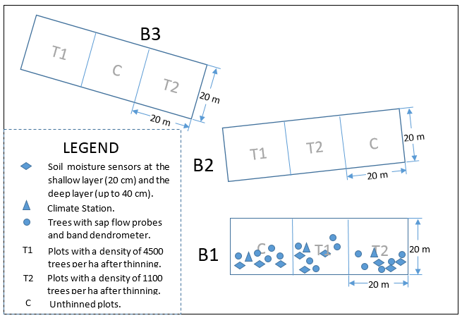 Fig. 2 A simplified graph of the three blocks
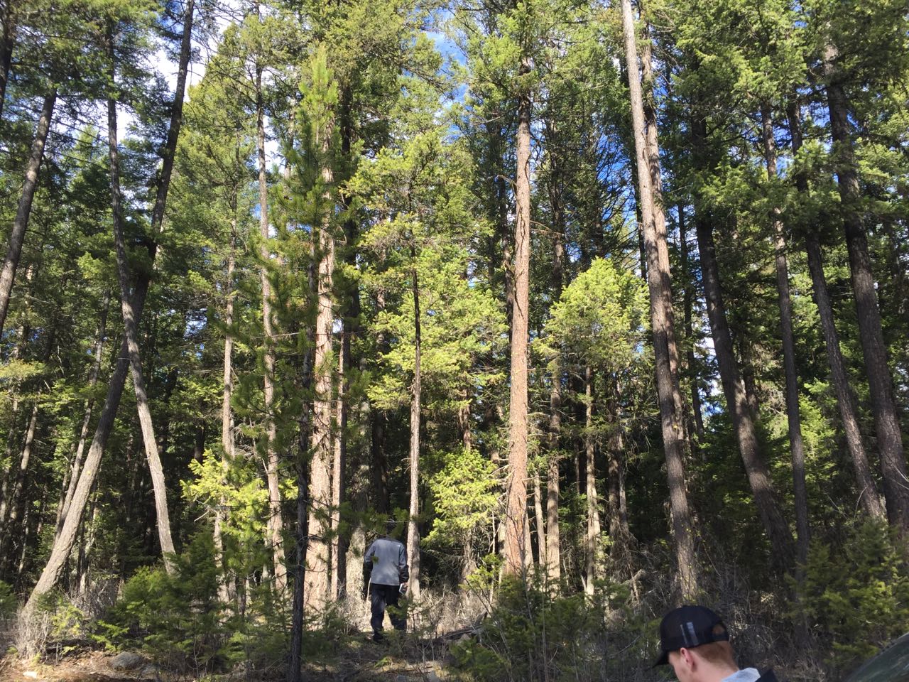 Figure 1. Forests around Postill Lake.
 Figure 2. Forests in the Upper Penticton Watershed. (Pink frame indicates the potential experimental site)
 Figure 3. Forests in the Mrya Canyon Trestles.