The distribution of precipitation in both space and time is typically skewed to the right. Since precipitation data cannot be expected to be normally distributed, the concept of variance has limited meaning for raw precipitation data. This raises the question of whether it is valid to use raw precipitation data within a principal components analysis (PCA), which is a variance-based technique. In this note, I evaluate this problem from both a statistical and ecological perspective.

The statistical rationale for transformation of precipitation variables towards a normal distribution prior to PCA is to facilitate a meaningful quantification of variance, and to stabilize the variance (reduce heteroskadacity). The ecological rationale for transformation of precipitation is that the meaning of the units changes across the range of values. For example, the ecological effect of a 100mm difference in annual precipitation is very different if the reference climate is 200mm vs 2000mm. Failing to transform precipitation variables may have profound implications for principal components analysis, because ecologically important variation at small precipitation values will be under-emphasized relative to ecologically less relevant variation at large values.

I have been surprised by the ambiguity surrounding whether or not data normality is an assumption of PCA. However, the predominant textbooks on PCA generally (Jolliffe 2002) and in the atmospheric sciences specifically (Wilks 2006) argue that PCA does not require multivariate normality of the data except for calculating inferential statistics on the PCs. Many sources informally state that normality is a “nice-to-have” for PCA, without explaining the implications of non-normal input data. Transformation of variables towards symmetric or normal distributions prior to PCA is a common practice (e.g. Wold et al. 1987, Baxter 1995) especially with regards to precipitation (e.g. Comrie and Glenn 1998, Hamann and Wang 2006).

Both Jolliffe (2002) and Wilks (2006) emphasize the critical importance of scaling the input variables so that their variance relative to each other is meaningful. It seems logical that this consideration could be applied to ensuring that the meaning of the data units is consistent throughout the range of the data in any given variable.  The distribution of the data affects the direction (eigenvectors) and magnitude/rank (eigenvalues) of the principal components. Hence the distribution of each variable should be meaningful in the context of linear analysis. As mentioned previously, the ecological meaning of the raw units of precipitation (e.g. mm) depends on the reference condition (e.g. 200 vs. 2000 mm). a power transformation (e.g. log-transformation) is widely recommended to make the units of precipitation scale-dependent (e.g. Wilks 2006).

This post explores the effect of transformation on PCA using an example data set.

Methods

The data for this analysis is 1951-2000 climate normals compiled from CRU TS3.21 gridded data (Harris et al. 2013) for North America (Figure 1). I’ve also created 6 regional subsets of the data to help with interpretation of the graphs. Monthly temperature and precipitation were converted to the 19 Bioclim variables using the biovars {dismo} call in R.

Figure 1: Extent of the North American study area used in this analysis, including the extents of the regional subsets.

Results

The distributions of 1951-2000 precipitation normals across North America are heavily skewed to the right (Figure 2). Log-transformation renders the distributions approximately symmetrical, though residual skewness in variables 14, 17, and 18 indicates that these variables are not log-normal and that adjusting the power transformation would be required to achieve symmetry.

Figure 2: histograms of raw and log-transformed Bioclim precipitation normals for the north American study area. (BIO12 = Annual Precipitation; BIO13 = Precipitation of Wettest Month; BIO14 = Precipitation of Driest Month; BIO16 = Precipitation of Wettest Quarter; BIO17 = Precipitation of Driest Quarter; BIO18 = Precipitation of Warmest Quarter).

The effect of the skewness on the relationship between precipitation and temperature is illustrated in Figure 3. In the absence of transformation, the dispersion of the data is dominated by wetter climates. Log-transformation provides much greater resolution of the differences between moderate, dry, and very dry climates. However, it is not clear whether the principal component of this relationship would be substantially different in either data set.

Figure 3: scatterplots of raw and log-transformed annual precipitation against mean annual temperature across North America.

PCA on the full set of 19 variables (Figure 4) suggests that transformation doesn’t have a major effect on the first two principal components: the differences between the correlations with the raw variables (red arrows) are only subtle in the two plots. However, scree plots (Figure 5) indicate that regional variance is partitioned quite differently in the two analyses, suggesting that there may be important differences in the third through sixth principal components.

Figure 4: two-dimensional climate space of North America, showing correlation vectors with the BioClim variables (left) and the subspaces occupied by the regional subsets of the data.

Figure 5: Scree plots of the North American PCA using raw and log-transformed precipitation, showing the proportion of total variation explained by each PC for the whole continental data set (grey line) and for regional subsets of the data.

Conclusions

It seems to be generally accepted that normality of input variables is not an assumption of PCA, unless inferential statistics are to be derived from the principal components. However, precipitation variables typically follow a heavily skewed gamma distribution, and transformation towards a normal distribution is a common practice to provide a more meaningful description of the data from both a statistical and ecological perspective. It is expected that transformation will influence the direction and magnitude of the principal components. However, the results of this case study indicated that the effect of transformation on the PCA was only subtle. There doesn’t appear to be an unequivocal requirement for transformation of precipitation data prior to PCA if subsequent analyses of the principal components do not require normality. Nevertheless, transforming precipitation data towards normality prior to PCA is highly recommended as a best practice.

References

Baxter, M. J. 1995. Standardization and Transformation in Principal Component Analysis, with Applications to Archaeometry. Journal of the Royal Statistical Society 44:513–527.

Comrie, A. C., and E. C. Glenn. 1998. Principal components-based regionalization of precipitation regimes across the southwest United States and northern Mexico , with an application to monsoon precipitation variability. Climate Research 10:201–215.

Hamann, A., and T. Wang. 2006. Potential Effects of Climate Change on Ecosystem and Tree Species Distribution in British Columbia. Ecology 87:2773–2786.

Harris, I., P. D. Jones, T. J. Osborn, and D. H. Lister. 2013. Updated high-resolution grids of monthly climatic observations – the CRU TS3.10 dataset. International Journal of Climatology 34:623–642.

Jolliffe, I. T. 2002. Principal Component Analysis, Second Edition. Page 487. Springer, New York.

Wilks, D. S. 2006. Statistical Methods in the Atmospheric Sciences, Second Edition. Page 627. Internatio. Academic Press.

Wold, S., K. Esbensen, and P. Geladi. 1987. Principal component analysis. Chemometrics and Intelligent Laboratory Systems 2:37–52.

Excerpts from the literature

Jolliffe (2002):

We digress slightly here to note that some authors imply, or even state explicitly, as do Qian et al. (1994), that PCA needs multivariate normality. This text takes a very different view and considers PCA as a mainly descriptive technique. It will become apparent that many of the properties and applications of PCA and related techniques described in later chapters, as well as the properties discussed in the present chapter, have no need for explicit distributional assumptions. It cannot be disputed that linearity and covariances/correlations, both of which play a central role in PCA, have especial relevance when distributions are multivariate normal, but this does not detract from the usefulness of PCA when data have other forms.

The distributional results outlined in the previous section may be used to make inferences about population PCs, given the sample PCs, provided that the necessary assumptions are valid. The major assumption that x has a multivariate normal distribution is often not satisfied and the practical value of the results is therefore limited. It can be argued that PCA should only ever be done for data that are, at least approximately, multivariate normal, for it is only then that ‘proper’ inferences can be made regarding the underlying population PCs. As already noted in Section 2.2, this is a rather narrow view of what PCA can do, as it is a much more widely applicable tool whose main use is descriptive rather than inferential. It can provide valuable descriptive information for a wide variety of data, whether the variables are continuous and normally distributed or not. The majority of applications of PCA successfully treat the technique as a purely descriptive tool, although Mandel (1972) argued that retaining m PCs in an analysis implicitly assumes a model for the data

Wilks (2006):

The distribution of the data x whose sample covariance matrix [S] is used to calculate a PCA need not be multivariate normal in order for the PCA to be valid. Regardless of the joint distribution of x, the resulting principal components ‘u_m will uniquely be those uncorrelated linear combinations that successively maximize the represented fractions of the variances on the diagonal of [S].

Comrie and Glenn (1998):

Pearson’s correlation coefficient used in the PCA input matrix can be sensitive to non-normality (White et al. 1991). In practice, PCA seems quite robust to moderate departures from normality of input data, but given the unusual precipitation distributions in some parts of the study area (especially stations with many zero precipitation months in the record), it seemed prudent to evaluate the regionalization using data transformed somewhat closer to normal. We examined frequency distributions across stations and experimented with several transformations, including the gamma distribution that is bounded on the left by zero and positively skewed, and therefore used in some precipitation studies. However, a simple square root transformation of monthly precipitation (p) appeared most useful when considered across all stations (i.e. p0.5).

Baxter (1995):

The logarithmic transformation, to base 10, of data before a principal component or other analysis is common. One reason for this is a belief that, within the raw materials of manufacture, elements have a natural log-normal distribution, and that normality of the data is desirable. A second reason is that a logarithmic transformation tends to stabilize the variance of the variables and would thus give them approximately equal weight in an unstandardized principal component analysis. A third reason sometimes cited is that, empirically, the use of a logarithmic transformation leads to more satisfactory results. In advocating the use of logarithmic transformation early work at the Brookhaven Laboratory has been influential (Bieber et al., 1976; Harbottle, 1976). Not everyone has been persuaded and a discussion of the issues involved and debate, with references, was given by Pollard (1986).

Wold et al. (1987):

Second, the data matrix can be subjected to transformations that make the data more symmetrically distributed, such as a logarithmic transformation, which was used in the swedes example above. Taking the logarithm of positively skewed data makes the tail of the data distribution shrink, often making the data more centrally distributed. This is commonly done with chromatographic data and trace element concentration data.

Summary

This post explores the effects of the so-called “curse of dimensionality” on Mahalanobis distance metrics. In simulated and real data, I demonstrate that the meaning of Mahalanobis units changes with increasing dimensionality: observations recede away from any reference coordinate due to the progressive exclusion of data space from the unit sphere. The result is that Euclidean and Mahalanobis distance units do not provide a direct measure of probability density in more than one dimension. It turns out that these dimensionality effects are the essence of the statistical theory of the chi-square distribution.  A meaningful distance/dissimilarity metric can be created by dividing distance by the square root of the dimensionality of the data space, which appears to create a reasonably intuitive metric based on the probability density of multivariate normal data.

Introduction

The premise of my research so far has been that the historical range of interannual climatic variability provides an ecologically meaningful metric of climatic differences over space and time. Building on the standardized Euclidean distance approach of Williams et al. (2007), I have developed a Mahalanobis metric based on the average standard deviation of historical interannual climatic variability across representative locations in any given study area. My intent is to use this metric to measure the degree to which future climatic conditions differ from those found in the current climatic classification. in other words, I intend to use the standard deviation of the historical range of variability as a unit of distance between future conditions and present conditions.

The first indication that something was missing from this approach was when I made maps of the distance from 1971-2000 normals to the 1971-2000 normals for a single location representing a BEC variant. For example, in the climatic distance map for the CDFmm (Figure 1), a very limited area is within 1 unit of the centroid, and most of the CDFmm is outside 2 units. If 1 M unit represents a standard deviation of temporal climatic variability, I would have expected most of the climate normals in the Georgia Basin to be within 2, if not 1, standard deviations from the centroid location.

Two reasons came to mind for the apparent overestimation of climatic distance: The first potential reason is overfitting. I used 10 principal components, and I standardized all the PCs to achieve a Mahalanobis metric. Given that the 10^th PC is given the same weight as the first, some amount of overfitting might be expected. However, I demonstrated in my last post that overfitting due to retained dimensions was not apparent in climate year classification results. Furthermore, adding dimensions with low spatial variability should reduce a Mahalanobis dissimilarity estimate, i.e. do the opposite to what seems to be the problem. The other possible reason is the “curse of dimensionality.” I looked into it, and it turns out that my thinking about distance was neglecting some fundamental geometric realities.

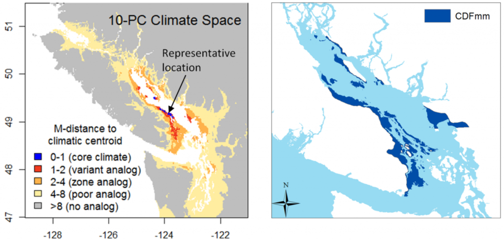
Figure 1: Mahalanobis distance from the 1970-2000 climatic normals in the Pacific Northwest to a location representing the average climate of the CDFmm.

How does the map change with different numbers of PCs?

The obvious firsts step is to see how the map changes at different levels of dimensionality (numbers of PCs retained) (Figure 2). One principal component is obviously too little information: false analogues are abundant in the interior rainshadow. The 2-PC climate space yields much better results, as would be expected because there is another key dimension of climatic variability to measure distance in. The 4 and 10-PC climate spaces show the core areas becoming progressively more distant, even though the outer limits of the range of analogues contracts only subtly. Given that my previous posts have demonstrated that the spatial variation in climate is predominantly captured in the first three PCs, this non-proportionate “distancing” phenomenon is suspect.

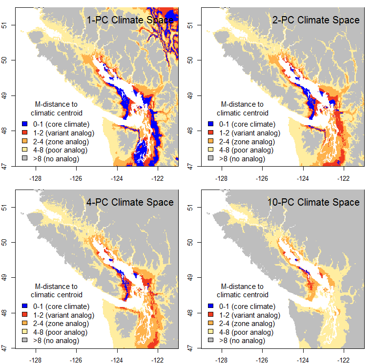
Figure 2: climatic distance to the CDFmm climatic centroid at different levels of dimensionality.

Another way to see the effect of dimensionality is in histograms of the distance of individual climate years to their own centroid (Figure 3). In one dimension, the distance to centroid takes the expected half-normal distribution, in which most climate years are within one M unit (i.e. one standard deviation) of their centroid, and almost all are within two M units. However, this distribution becomes altered in climate spaces of more than one dimension. The distances to centroid increase at higher dimensions, to the extent that in 10 dimensions there are no climate years within 1 M unit of the reference condition (i.e. the origin of the climate space). This indicates that the meaning of distance and probability density changes with increasing dimensionality.

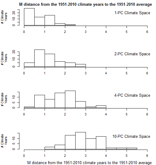
Figure 3: effect of dimensionality on the Mahalanobis distance of CDFmm 1951-2010 climate years to their own centroid.

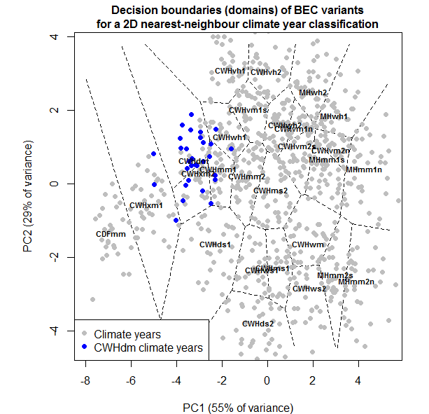
The shift in the distribution of distances between the mean of a sample and its observations has a very simple and intuitive geometric cause. Figure 4 is a plot of the CDFmm climate years in the first two PCS. By definition, about two-thirds of climate years lie within one standard deviation of PC1 (the area shaded gray). However, in two-dimensional space, a much smaller proportion of climate years are within a distance of one M unit of the centroid, i.e. within the unit circle. It follows that in three dimensions, even fewer observations would be within the unit sphere.

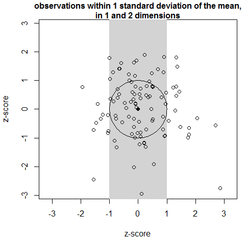
Figure 4: 2D demonstration of the reason for the exclusion of observations from the region of 1 standard deviation around the mean.

Simulations

The relationship between distance, probability density, and dimensionality can be explored through simple simulations of random data. The first simulation is simply a multivariate normal distribution with a standard deviation of one in each of i dimensions. At dimensionality higher than one, distances to centroid rapidly approach a Gaussian-like distribution with a standard deviation of 0.707 (square root of 2). This distribution is maintained at dimensionality higher than 3, even though the distance from the centroid increases. As a result, the ratio of the distance to centroid of the closest and furthest observations approaches 1 at very high dimensionality. The explicit description of this effect is generally attributed to Beyer et al. (1999).

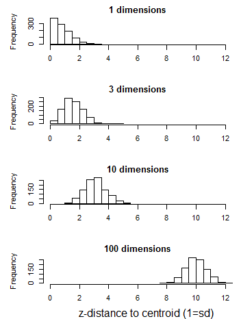
Figure 5: distance of observations of a simulated random normal sample (N=1000, sd=1) from their own centroid.

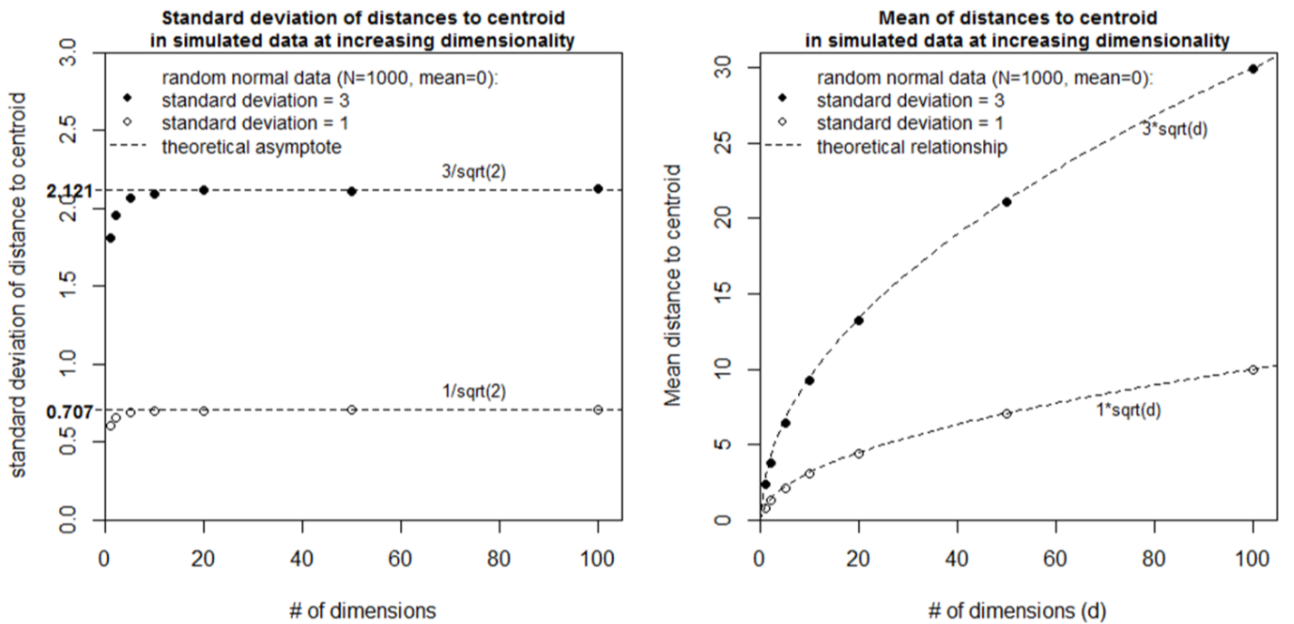
Simulation 2 explores the case of two random normal samples with the same centroid but different standard deviations (Figure 6). Although the two samples overlap in low dimensional space (<4 dimensions), they diverge from the mean (the origin) at different rates such that they are completely separate in high dimensional space. The standard deviation of distances to centroid is the standard deviation of the univariate data distribution divided by the square root of two (Figure 7). The mean distance to centroid is standard deviation of the data multiplied by the square root of the dimensionality.

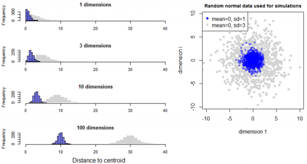
Figure 6: Simulation 2—Effect of dimensionality on distance to centroid in random multivariate normal data with the same mean but different standard deviations.

Figure 7: Simulations used to infer geometrical relationships between dimensionality and the distribution of distances to centroid.

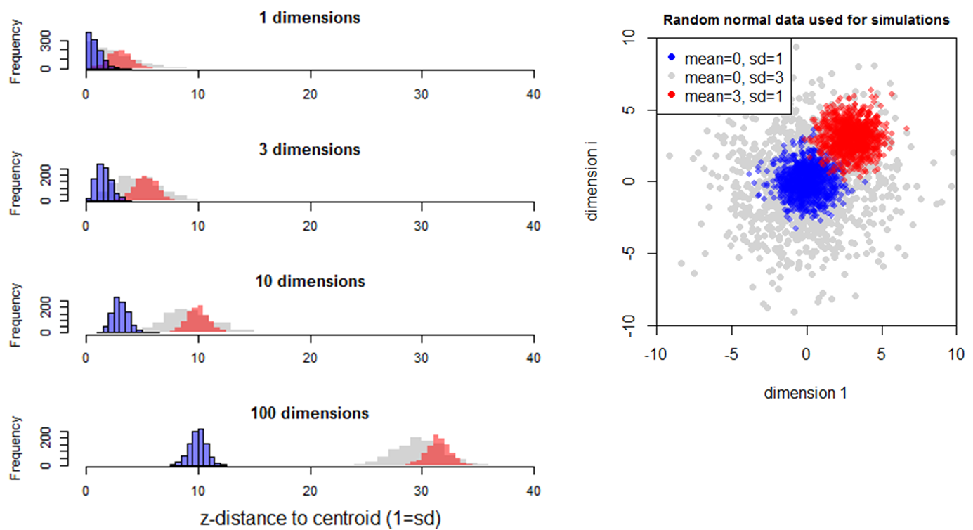
Simulation 3 adds an additional multivariate normal sample with a standard deviation of 1 and a mean of 3 in all dimensions (Figure 8). The distance from the origin to these observations (red distribution) is slightly greater than that of the multivariate normal sample with a mean of zero and standard deviation of 3 (grey distribution), though the mathematical relationship is not immediately clear. The standard deviation of the red sample is slightly less than one (0.98) in all levels of dimensionality. This is likely because the tail of the univariate distribution of this sample crosses the origin, resulting in a slightly folded distribution of distances to the origin. Nevertheless, this simulation indicates that dispersion (standard deviation of samples) is preserved in multidimensional distances.

Figure 8: Simulation 3—Effect of dimensionality on distance to an additional multivariate normal sample with a standard deviation of 1 and a mean of 3 in all dimensions.

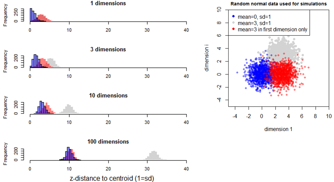
The last simulation investigates the effect of a sample mean being different in only one of many dimensions (Figure 9). In this case, the mean of distances of the different sample (red) approaches that of the reference sample (blue) in higher dimensionality. In other words, the distance between samples is influenced by the number of dimensions in which the difference between the samples occurs.

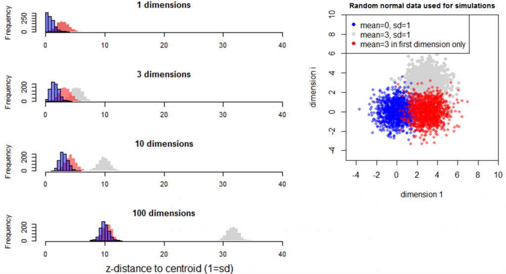
Figure 9: Simulation 4—Effect of dimensionality on distance to the origin in random samples with the same standard deviation but different means. The red sample has a mean of 3 in the first dimension, and a mean of zero in all other dimensions.

The simulations suggest the following attributes about the relationship between distance, probability density, and dimensionality:

• The relationship between distance and probability density is non-stationary under varying dimensionality. i.e. the probability of an observation occurring within a distance of one standard deviation of the sample mean decreases as the dimensionality increases.
• The probability distributions of multivariate normal data are hollow hyperspheres. The mean of the hyperspherical probability distribution is located at a distance from the centroid equaling the standard deviation of the multivariate normal data multiplied by the square root of the dimensionality. The standard deviation of the hyperspherical probability distribution is equal to the standard deviation of the multivariate normal data divided by the square root of two.
• The overlap between probability density distributions of multivariate normal data with different dispersion (i.e. different standard deviations) approaches zero with increasing dimensionality. In other words, given two different samples of the same mean but different standard deviations, the probability that observations from these two samples could occur in the same location approaches zero as dimensionality increases.
• The dispersion of probability density is preserved in high-dimensional space.
• The influence that the data distribution in any one dimension has on the total probability density of distance to centroid decreases with increasing dimensionality.

The geometrical phenomena described above are the essence of the statistical theory of the chi-square distribution. The squared Euclidean distance of standard (i.e. unit variance) multivariate normal data to their own centroid approach a chi-square distribution with degrees of freedom equalling the dimensionality of the data space (Wilks 2006). It follows that the squared Mahalanobis distance to centroid of any multivariate normal distribution will follow a chi-square distribution.

The effects of dimensionality on distance have also been studied in the data mining literature (e.g. Brin 1995, Beyer et al. 1999, Aggarwal et al. 2001), though often without recognition of the link to the chi-square distribution. In this context, they are typically referred to as an aspect of the “curse of dimensionality”, which refers to the exponential increase in data sparsity with increasing dimensionality.

Dimensionality effects are not discussed in the original formulation of the Standardized Euclidian Distance (SED) metric of novel and disappearing climates (Williams et al. 2007) nor in its regional applications (Veloz et al. 2011, Ackerly 2012, Ordonez and Williams 2013), even though dimensionality is likely an important determinant of the novelty threshold (SED_t) that is central to the metric.

Dimensionality effects in the spatiotemporal climate space of the BEC system.

How do these dimensionality effects play out in the spatiotemporal data set I am using for my analysis? A distance histogram of BC climates relative to the CDFmm variant (Figure 10) is quite revealing.

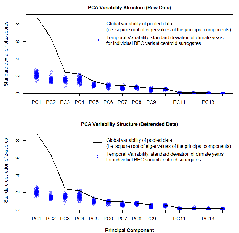
The mean of the probability distribution of CDFmm climate years is approximately the square root of the dimensionality. This would be expected, since the purpose of spatiotemporal standardization is to normalize temporal variability at each BEC variant centroid to approximate multivariate normality with a standard deviation of one. However, the distance to other BEC variants is relative stable at dimensionality more than two. The reason for this is likely because the first two PCs contain the vast majority of the spatial variation of the data (Figure 11). The other dimensions primarily represent different modes of temporal climatic variation, and therefore all variation in these lesser dimensions has approximately unit standard deviation. The result is that the relative distance between CDFmm climate years and those of other BEC variants decreases at higher dimensionality.

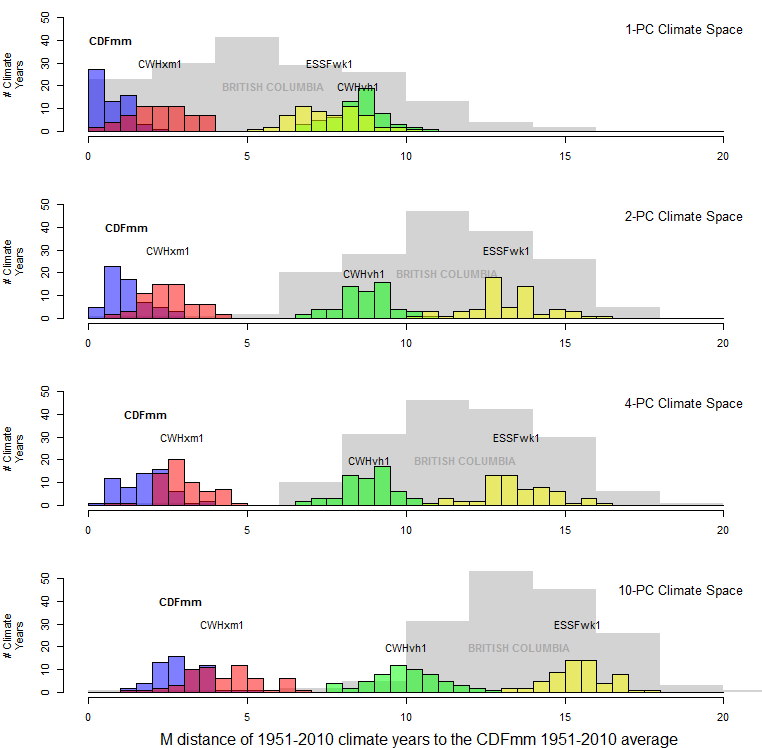
Figure 10: distance to the centroid of the CDFmm 1951-2010 climate years. Coloured histograms are 1951-2010 climate years for BEC variants representing similar (CWHxm1), somewhat different (CWHvh1), and very different (ESSFwk1) climates. The grey histogram is the distribution of 1971-2000 climate normals for 168 BEC variant representative locations.

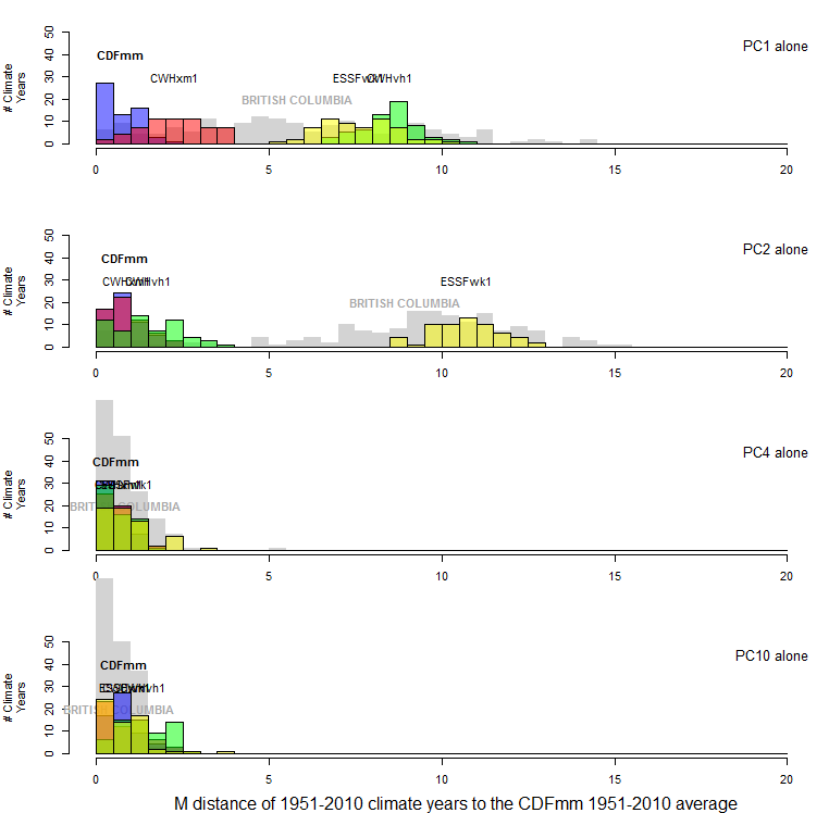
Figure 11: One-dimensional distance to the centroid of the CDFmm 1951-2010 climate years, for selected principal components. Coloured histograms are 1951-2010 climate years for BEC variants representing similar (CWHxm1), somewhat different (CWHvh1), and very different (ESSFwk1) climates. The grey histogram is the distribution of 1971-2000 climate normals for 168 BEC variant representative locations.

A solution: Dimensionality-adjusted Mahalanobis distance

My main interest in the relationship between distance, probability density, and dimensionality is in finding a good way of measuring differences between climatic conditions.  My goal is to achieve a unit of distance in climate space that reflects the scale of interannual climatic variability at any given location. the problem with the dimensionality effects is that they distort the meaning of the distance metric in terms of the probability density of variability around a reference condition. One way to correct for this aspect of the problem is to standardize distances so that the probability distribution of the interannual variability in climate-year distances from the climate normal of the reference location has a mean of one at any level of dimensionality.

Spatiotemporal PCA (stPCA) creates a data space in which the reference period climate years at selected locations follow an approximately standard multivariate normal distribution, assuming normality of the raw variables. As a result, the squared distances of the climate years to their average (the reference normal) follow a chi-square distribution with degrees of freedom equalling the dimensionality of the data space. The mean of the standard chi-square distribution equals the degrees of freedom and thus the dimensionality. Hence, dividing distances by the square root of the dimensionality will center the climate years for any location at a value of one. Further, the units of this dimensionality adjusted distance metric are interpretable as the standard deviations of spherical multivariate normal distributions. Compared to unadjusted distance, this metric appears to be more easily interpreted because it is intuitively related to univariate dispersion.

Figure 12 illustrates the effect of standardizing distances in climate space by the square root of the dimensionality. This standardization has the desirable effect of limiting the probability distribution of the climate years for the focal geographic location (the CDFmm in this case) to a mean of one. It also has the effect of compressing the distributions of other BEC variants as dimensionality increases. This compression is a result of there being little spatial variation in dimensions above the third PC (Figure 11), i.e. all BEC variants have the same mean in these lesser eigenvectors. Hence the average dispersion of the data declines with increasing dimensionality. Adding dimensions for which all group means are the same will make the groups appear more similar, and thus reduce the distances between them. This is a much more intuitive result than the unadjusted Mahalanobis distance.

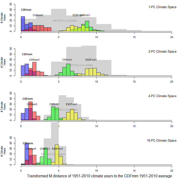
Figure 12: Effect of transforming distances to the CDFmm centroid by dividing them by the square root of the dimensionality. This transforms the Mahalanobis metric into units of standard deviations of multivariate normal data

Chi-square percentiles as an alternate distance metric

Since squared distances of climate years to their own average are expected to follow a chi-square distribution, it is logical that climatic dissimilarity could be measured in chi-square percentiles. This approach is demonstrated in Figure 13. Chi-square percentiles clearly provide a statistically precise distance metric. However, the horizon of the metric is very close to the origin: even a climate as similar to the CDFmm as the CWHdm is beyond the 99.99^th percentile. This likely limits the utility of chi-square percentiles for climate change analysis.

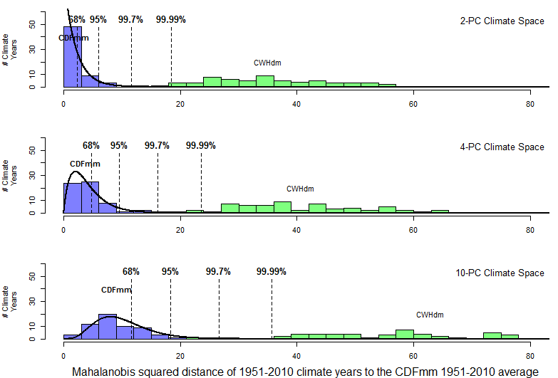
Figure 13: Utility of chi-square percentiles as a dimensionality-independent distance metric. The squared Mahalanobis distances of climate years to their own centroid follow a chi-square distribution, the percentiles of which provide a statistically precise distance metric. The horizon of this distance metric, however, is very short.

Distinction between distances to climate year distributions vs climate normals

When using the dimensionality-adjusted Mahalanobis distance as a dissimilarity metric, it is important to be mindful of the distinction between distances to climate year distributions vs climate normals. This is the distinction between the mean distance to a set of observations vs. the distance to the mean of those observations. As the mean of a standard multivariate normal distribution approaches a reference point, the distance between these two points will obviously approach zero.  However, the mean dimensionality-adjusted Mahalanobis distance from any reference point to standard multivariate normal data can never be less than one, because of the inherent dispersion of the data (Figure 14). It follows from this simple logic that a distance of one has different meanings for climate year distributions vs. climate normals.

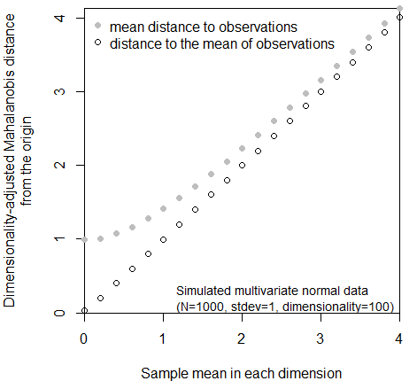
Figure 14: distinction between the mean distance to observations in a sample, as opposed to the distance to the mean (centroid) of the sample. This relationship is independent of dimensionality.

References

Ackerly, D. D. 2012. Future Climate Scenarios for California: Freezing Isoclines, Novel Climates, and Climatic Resilience of California’s Protected Areas. Page 64.

Aggarwal, C. C., A. Hinneburg, and D. A. Keim. 2001. On the Surprising Behavior of Distance Metrics in High Dimensional Space. Pages 420–434 Lecture Notes in Computer Science.

Beyer, K., J. Goldstein, R. Ramakrishnan, and U. Shaft. 1999. When is “Nearest Neighbour” Meaningful? Int. Conf. on Database Theory.

Brin, S. 1995. Near Neighbor Search in Large Metric Spaces. Pages 574–584 Proceedings of the 21st VLDB Conference. Zurich, Switzerland.

Ordonez, A., and J. W. Williams. 2013. Projected climate reshuffling based on multivariate climate-availability, climate-analog, and climate-velocity analyses: implications for community disaggregation. Climatic Change 119:659–675.

Veloz, S., J. W. Williams, D. Lorenz, M. Notaro, S. Vavrus, and D. J. Vimont. 2011. Identifying climatic analogs for Wisconsin under 21st-century climate-change scenarios. Climatic Change 112:1037–1058.

Wilks, D. S. 2006. Statistical Methods in the Atmospheric Sciences, Second Edition. Page 627. Internatio. Academic Press.

Williams, J. W., S. T. Jackson, and J. E. Kutzbach. 2007. Projected distributions of novel and disappearing climates by 2100 AD. Proceedings of the National Academy of Sciences of the United States of America 104:5738–42.

Summary

In this post, I use cross-validated climate year classifications to compare the effectiveness of linear discriminant analysis (LDA) vs. nearest neighbour classification on spatiotemporally standardized principal components (ST PCA). Despite achieving lower correct classification rates on training data, ST PCA performed as well as LDA on test data. This supports theoretical reasoning that ST PCA should be less prone than LDA to overfitting due to the structure of its eigenspace. Neither method showed evidence of overfitting at high dimensions, a perplexing result that deserves further consideration. These results suggest that the benefits of ST PCA over LDA—i.e. a more logical climate space for climate change analysis—do not come at the cost of lower classification effectiveness.

Introduction

In previous posts, I developed the methodology of spatiotemporal standardization (STS) as a way of structuring the climate space of British Columbia around historical variability and the differences between BEC variants. Doing STS on the raw data, and again on truncated principal components creates a climate space in which nearest-neighbour classification is similar to classification via linear discriminant analysis (LDA). Nevertheless, I found that LDA was somewhat more effective at climate year classification in training data, and thus possibly more desirable for classification of future climates. The purpose of this post is to do a first pass on cross-validated comparison of LDA and what for the moment I am calling spatiotemporal principal components analysis (ST PCA).

Classification Methods

The data for this analysis is a 1961-1990 time series of 14 annual variables at each of 168 BEC variant centroid surrogates. This is data from ClimateWNA v4.72.

Both methods use nearest-neighbour classification (k=1). Each 14-variable climate year is classified by assigning it to the nearest BEC variant 30-yr normal. The only difference between the two methods is the eigenspace in which this Euclidian measure is performed.

The eigenspace for the LDA is calculated using the “lda” call in the MASS package of R. This call extracts eigenvectors based on the ratio of between-group to within-group scatter, then standardizes the eigenvectors to unit within-group variance. I have confirmed that nearest neighbour classification in this eigenspace produces identical results to the classification produced by the predict(lda) call.

The eigenspace for the ST PCA is created by the following process: (1) standardizing the 14 raw climate variables by the average standard deviation of temporal variability of each BEC variant; (2) PCA using the “prcomp” call in the MASS package of R; and (3) standardizing retained eigenvectors by the average standard deviation of temporal variability of each BEC variant. The first round of standardization has the effect of supervising the PCA so that it selects eigenvectors with a high ratio of spatial (between-group) to temporal (within-group) variation. The second round of standardization removes the influence of redundant and correlated variation in the raw data, and appears to be similar to the eigenvector standardization performed by the “lda” call.

Cross-validation methodology

Two measures are taken to reduce the influence of spatial and temporal autocorrelation on the cross-validation results, using the “xval.buffer” method of the CaDENCE package in R (Cannon 2012). First, spatial autocorrelation is addressed by testing against blocks of the same three contiguous years in all BEC variants. Second, serial autocorrelation is addressed by a three-year buffer on the test data: i.e. 3 years on either side of the test data are withheld from the training data. There are 10 iterations of cross-validation over the 30-yr classification period, as illustrated in Figure 1.

Figure 1: illustration of buffered cross-validation using test data composed of contiguous blocks of three years, using the “xval.buffer” method of the CaDENCE package in R (Cannon 2012).

The meaning of “correct” in climate year classification

Supervised classification methods such as LDA are based on the principle of training the classification model with data of known class, and validating the model with test data of known class. In this typical context, the skill of the model is inferred from “correct classification rate”: the proportion of the test observations that are assigned the correct known class. In the context of climate year classification, there is no true “correct” classification:  the a priori class of each climate year is the spatial location of the observation (e.g. BEC variant centroid surrogate), and the assigned class is the climatic condition (e.g. 30-yr normal) that the climate year most closely resembles. “correct classification rate” in this context depends both on the ability of the model to differentiate the groups, and on the intrinsic differention (degree of overlap) between the groups. For this reason, “differentiation” is a more precise term for correct classification rate in climate year classification.

Results

As demonstrated in previous posts, LDA achieves higher differentiation in the training data than ST PCA (Figure 2). However, both methods achieved similar differentiation in the test data, suggesting that ST PCA and LDA are equally effective as climate year classification methods. Overfitting due to dimensionality is not apparent: differentiation in the test data declined only very slightly when more than ten eigenvectors were retained for classification. Cross-validated differentiation of individual BEC variants is equivalent for both methods (Figure 3).

Figure 2: cross-validated climate-year differentiation skill of LDA and ST PCA, for increasing dimensionality of eigenspaces.

Figure 3: cross-validated climate-year differentiation skill of LDA and ST PCA, showing the distribution of differentiation rates for each of the 168 BEC variants. Both classifications used 10 eigenvectors.

Discussion

Prior to this analysis, I expected LDA to be more prone to overfitting because selecting eigenvectors based purely on the ratio of between-group to within-group variance allows eigenvectors with low variance to be assigned moderate rank. ST PCA is likely more robust to overfitting because it prioritizes between-group variation while still ranking eigenvectors based on variance. This analysis suggests that LDA is indeed more prone to overfitting than ST PCA. The extent of overfitting in LDA was such that both methods have equivalent differentiation skill on the test data, despite better differentiation by LDA on the training data. This suggests that the other advantages of ST PCA over LDA, e.g. its more logical eigenvector structure, do not come at a cost in terms of classification skill.

The lack of overfitting at high dimensions is perplexing. I expected to see a dramatic decline in cross-validated skill of both methods when more than 10 eigenvectors were retained. Both methods standardize the retained eigenvectors to unit within-group variance. The effect of this standardization is to make all retained eigenvectors the same importance in the classification. It would seem logical that inflating the variance of dimensions with no discriminating power would confound the distance metric used for classification. I would also expect that the addition of these trivial dimensions would begin to invoke the curse of dimensionality, in which all observations seem equally distant from any given point in high-dimensional space. Neither of these effects are apparent, and the failure of this logic warrants further consideration.

Independent test data are essential for reliable model validation.  This is problematic for climate year classification, since the cross-validated skill of classification models is inflated by serial autocorrelation of time series data (Shabbar and Kharin 2007). The problem of finding independent data is exacerbated by the fact that there is no a priori class of a climate year, and thus no definitive means of declaring a classification as “correct”. However, the objective of this analysis is to compare the differentiating skill of LDA and spatiotemporal PCA, rather than to assess the absolute skill of either method. Imperfectly independent test data are likely to be adequate to assess the relative effectiveness of the methods.

References

Cannon, A. J. 2012. Neural networks for probabilistic environmental prediction: Conditional Density Estimation Network Creation & Evaluation (CaDENCE) in R. Computers & Geosciences 41:126–135.

Shabbar, A., and V. Kharin. 2007. An assessment of cross-validation for estimating skill of empirical seasonal forecasts using a global coupled model simulation. CLIVAR Exchanges 12:10–12.

Summary

A meaningful metric of climatic difference is helpful for climate change analysis. There is a strong statistical and ecological rationale for the use of Mahalanobis metrics in multivariate analysis of climatic novelties, since it removes the effect of correlations and trivial redundancies between climate variables. This post describes standardization of eigenvectors on the temporal component of spatiotemporal data. In other words, this method performs a second round of spatiotemporal standardization on features extracted from spatiotemporally standardized data.  This second standardization approach appears to be functionally (and possibly mathematically) equivalent to spherical normalization of the within-groups covariance matrix of extracted features, which is commonly used within linear discriminant analysis to improve classification. In addition to its advantages in classification, this method provides a Mahalanobis metric whose units reflect the average temporal variability of the study area. This “M-metric” is a robust and ecologically meaningful metric for quantification of climatic differentiation and change.

The rationale for standardization of extracted features

Standardization (a.k.a. scaling) is a very common procedure in multivariate analysis. The basic rationale for standardization is that different variables have different and incomparable units of measurement (e.g. ^oC vs. mm). However, even for variables with comparable units, there is an additional ecological rationale for standardization of interannual variability: life strategies of organisms will generally be adapted to the background variability of any given climate element. Adaptation to historical variability is expected to be both temporal (e.g. winter vs. summer temperatures) and spatial (e.g. mean annual temperature in temperate vs. tropical regions) (Mora et al. 2013). This ecological rationale for standardization must be considered in metrics for climatic differences in both space and time.

Standardization gives all variables equal or comparable variance, and thus equal a priori influence on the outcome of a principle components analysis (PCA). However, PCA aggregates the correlated variance of the raw variables into the extracted principal components. The relative variance of the principal components thus reflects the redundant variance in the raw variables. Addition of a trivially and perfectly redundant variable to the raw data (e.g. a second set of MAT values), will have the non-trivial result of increasing the variance of one of the principal components and possibly increasing its rank. This behaviour highlights the importance of careful variable selection prior to performing PCA. Nevertheless, correlation between raw climate variables is inevitable, and so the ecological meaning of the unequal variance of principal components needs to be considered.

Extracted features (e.g. principal components) represent independent (uncorrelated) dimensions of climatic variation. Regardless of whether unequal variance in the principal components is due to trivial redundancies or meaningful correlations, the relative scales of variation in the principal components are unlikely to be ecologically meaningful due to life strategy adaptation.  What is important is the magnitude of a climatic difference or change relative to the background variation of any given principal component. In this light, the ecological rationale for standardization of raw variables also applies to principal components and other eigenvectors extracted by other methods, such as LDA.

Mahalanobis distance vs. Euclidian distance

I have demonstrated in previous posts that principal components analysis doesn’t affect the distance between observations in climate space. Therefore, Euclidian distance on non-truncated principal components is the same as Euclidian distance on raw variables. Standardization of the principal components (dividing by the standard deviation of z-scores) creates a climate space in which Euclidean distance is equivalent to Mahalanobis distance in the standardized but unrotated climate space (Stephenson 1997).  The units of standardized eigenvectors (e.g. standardized principal components) therefore are Mahalanobis metrics. Similar to z-scores, the precise meaning of a Mahalanobis metric depends on how the eigenvectors are derived from the raw data (e.g. PCA vs. LDA) and how the standardization population is defined (e.g. global vs. spatiotemporal).

Spherization of temporal climate envelopes

As shown in the previous post, spatiotemporal standardization operates by dividing each observation by the average standard deviation of climatic anomalies across the study area. This approach creates temporal climatic envelopes that are approximately spherical, and collectively have an average standard deviation of one z-score. Climate envelopes of individual locations will be larger or smaller, and more-or-less spherical, depending on their variability in each climate element relative to the study area average. Principal components analysis of this space is desirable, since it aggregates redundant variation into uncorrelated dimensions of variation. However, the aggregation of variance into principal components creates ellipsoidal (oblong) temporal climate envelopes. As discussed above, the ecological meaning ellipsoidal shapes of temporal climate envelope is ambiguous.  A second round of spatiotemporal standardization of the principal components returns the temporal climate envelopes to an approximately spherical shape. This second standardization can be called “spherization of within-group variability,” or just “spherization” for simplicity.  The metric of the sphered climate space can be called the M-score, because it represents a unit of Mahalanobis distance based on the average standard deviation of temporal anomalies of z-scores over all locations in the study area. The process of spherization of truncated principal components is illustrated in Figure 1.

Figure 1: effect of spatiotemporal standardization of principal components (spherization) on the variability structure of the BEC variants of the south-central interior BC.

Figure 2: the role of spherization in linear discriminant analysis of the BEC variants of the south-central interior BC.

Comparison with linear discriminant analysis

Many aspects of the above procedure (spherization of local anomalies (within-group variability) of the principal components of spatiotemporally standardized data) are conceptually similar to the procedures of linear discriminant analysis. A comparison of the methods and results of the two procedures is warranted.

Spatiotemporal standardization expresses spatial variability between locations in terms of the average temporal variability of all locations. This is similar, though not equivalent, to the ratio of between-groups to within-groups scatter matrix that is the basis of LDA: The within-groups scatter matrix is the sum of the individual group covariance matrices, which is equivalent to the average covariance matrix, which in turn is likely equivalent in ratio form to the average matrix of standard deviations.  Variables that have higher spatial variability will have larger variance in a spatiotemporally standardized data set. A principal components analysis of spatiotemporally standardized data is therefore functionally similar to LDA, because both give high priority (eigenvalues) to variables with a high ratio of between-group to within-group variability.

Despite this functional similarity, PCA calculates eigenvalues of the total data variance, while LDA calculates eigenvalues of the ratios of between- to within-group variance. The extracted features are different as a result. Low-eigenvalues in PCA indicate residual dimensions with very low spatial and temporal variation (Figure 1).  Low eigenvalues in LDA indicate dimensions with low spatial variation, but which may nevertheless have substantial temporal variability (Figure 2). PCA is advantageous because it facilitates truncation of the features with very low variance; in Figure 1 it is clear that the last four principal components can be dropped from further analysis with minimal loss of information. However, beyond the process of truncation, the advantages of PCA vs. LDA are ambiguous. PCA structures the climate space in order of decreasing total variance, while LDA structures the climate space in order of decreasing spatial differentiation. Both of these structures are climatically and ecologically meaningful in their own way, and their relative advantages will depend on the specific research question being asked.

Effect of spherization on climate year classification

Spherization is not integral to the feature extraction component of the LDA procedure, but it is typically incorporated into LDA because it has an important role in classification. For example, it is an integral component of the lda{MASS} call in R. it is logical that spherization of the principal components should also improve nearest neighbour classification. Figure 3 demonstrates the sequential effects of spatiotemporal standardization and spherization on differentiation (nearest-neighbour correct classification rates) between BEC variant temporal climate envelopes. Typical global z-standardization produces an average differentiation in the otherwise untransformed climate space of 36%. Spatiotemporal standardization improves differentiation to 41%. As demonstrated previously, PCA has no effect on differentiation. However, spherization of the PCA improves differentiation to 47%. LDA, which includes spherization as part of its classification procedure, achieves a differentiation of 53%. It is notable that LDA without spherization (not shown in Figure 3) only achieves 44% differentiation. Spherization is clearly advantageous for classification. Spatiotemporal standardization followed by spherization of principal components achieves classification results that are only marginally poorer than LDA.

Figure 3: effect of spatiotemporal (ST) standardization and spherization on climate year classification of BEC variants, compared to simple “global” z-standardization (left) and linear discriminant analysis (LDA, right). All classifications use the nearest-neighbour criterion.

Use of spherization and Mahalanobis distance in the ecological literature climate change

Standardized anomalies are frequently used in the atmospheric sciences , and are useful for univariate analysis because they quantify variability in terms of standard deviations (z-scores). Mora et al. (2013) adapted the concept of standardized anomalies to describe “climate departures”, i.e. the year at which the future temporal climate envelope of any given location ceases to overlap with its own historical temporal climate envelope. Although they did univariate analysis on seven climate variables, they did not perform any multivariate analysis. This is very likely due to the purpose of their paper as a simple way to communicate climate change impacts to a large non-expert audience. Nevertheless, the high impact of this paper suggests that an equivalent multivariate approach is in demand.

Williams et al. (2007) provided a multivariate analysis of standardized anomalies, using a standardized Euclidean distance metric. The authors may have opted against a Mahalanobis metric for the sake of simplicity and ease of communication.  Nevertheless, standardized Euclidean distance metrics are susceptible to the unjustified influence of correlations in the input variables, and so are problematic for quantitative investigation of climate change.

Hamann and Wang (2006) used linear discriminant analysis on spatial variation in climate normals to define the climate envelopes of BEC variants for the purposes of climate change analysis. They explicitly noted that this method uses a Mahalanobis distance for climatic classification. This Mahalanobis metric is very similar to the one I have proposed because it is based on spherization of within-group variability. However, the units of the Mahalanobis metric in Hamann and Wang (2006) reflect the average spatial variation of climate normals within BEC variants, and thus the scale of BEC mapping. A Mahalanobis metric based on the temporal variation at individual locations is essentially independent of BEC mapping, which is likely preferable for subsequent analysis of BEC mapping.

As an alternative to discriminant analysis for species distribution modeling, Roberts and Hamann (2012) proposed nearest-neighbour classification using Euclidean distance of heavily truncated principal components. They claimed that this is a modified Mahalanobis distance, but do not specify any standardization of the principal components in their methodology. Euclidian distance on principal components is the same as Euclidian distance on raw variables. As a result, it does not appear that their method produces a Mahalanobis metric, though this needs to be verified.

References

Hamann, A., and T. Wang. 2006. Potential Effects of Climate Change on Ecosystem and Tree Species Distribution in British Columbia. Ecology 87:2773–2786.

Mora, C., A. G. Frazier, R. J. Longman, R. S. Dacks, M. M. Walton, E. J. Tong, J. J. Sanchez, L. R. Kaiser, Y. O. Stender, J. M. Anderson, C. M. Ambrosino, I. Fernandez-Silva, L. M. Giuseffi, and T. W. Giambelluca. 2013. The projected timing of climate departure from recent variability. Nature 502:183–7.

Roberts, D. R., and A. Hamann. 2012. Method selection for species distribution modelling: are temporally or spatially independent evaluations necessary? Ecography 35:792–802.

Stephenson, D. B. 1997. Correlation of spatial climate/weather maps and the advantages of using the Mahalanobis metric in predictions. Tellus 49A:513–527.

Williams, J. W., S. T. Jackson, and J. E. Kutzbach. 2007. Projected distributions of novel and disappearing climates by 2100 AD. Proceedings of the National Academy of Sciences of the United States of America 104:5738–42.

Summary

This post describes a modification of anomaly standardization for spatiotemporal climate data. I have not yet found an explicit description of this approach in the literature, so for the moment I am calling it spatiotemporal standardization. This method standardizes climate variables by the average standard deviation of interannual variability of all locations in the study area. It is a useful compromise between typical “global” z-standardization across the whole data set and anomaly standardization of each location’s interannual variability. Spatiotemporal standardization serves two important purposes for climate change analysis: (1) it provides an ecologically meaningful metric of climatic difference—the spatiotemporal z-score—that directly reflects observed interannual variability in each climate element; and (2) it supports PCA feature extraction that appropriately balances spatial (between-group) and temporal (within-group) variability. Unlike local anomaly standardization, spatiotemporal standardization does not distort the climate space: it preserves the relative distances between all observations within any given variable. However, it alters euclidean distance of the climate space by emphasizing variables with high spatial (between-group) variability, and therefore improves climate year classification results. Spatiotemporal standardization appears to be an effective foundation for analysis of bioclimate differentiation, historical variability, and degrees of climatic novelty.

Global, anomaly, and spatio-temporal standardization

Standardization is necessary for multivariate analysis of climate data because climatic elements (e.g. temperature and precipitation) have different units and scales (e.g. degrees Celsius and millimetres). Z-standardization subtracts the population mean from each observation, and then divides by the population standard deviation. This method reduces observations to z-scores, which have a mean of zero and unitless values representing standard deviations above and below the mean. Beyond the simple utility of standardization, the z-score is a useful concept for climatic analysis because it provides a metric of climatic difference that is directly related to the statistical variability of climate elements.

The z-standardization process can be customized for specific purposes by carefully defining the population.  The most common approach to z-standardization is to treat all observations in the data as one population. This approach can be called “global standardization”. The major disadvantage of global standardization for spatio-temporal data sets is that it returns z-scores that arbitrarily reflect the spatial variation of climate elements over the study area (a larger study area will have a larger range of variation), and which therefore have limited ecological meaning. An alternate approach is to apply standardization locally and temporally by defining the population as the annual observations at one location over a given time period. This is called anomaly standardization in the atmospheric sciences. Standardized anomaly z-scores are a measure of climatic difference in space or time in terms of the historical range of climatic variability at an individual location. Standardized anomalies thus provide an ecologically meaningful metric for climatic differences between locations, for the magnitude of climate change, and for analog goodness-of-fit. For example, anomaly standardization is the basis for the “standardized Euclidian distance” approach described by Williams et al. (2007) for their analysis of novel and disappearing climates.

One limitation of anomaly standardization is that it transforms climate data at each location by a different scalar, and therefore distorts the spatial structure of temporal variability in the study area. This removes important information from the data and precludes comparison of the relative magnitude of historical variability and future climate change at different locations. One solution to this problem is to standardize observations by the mean of the anomaly standard deviations in all locations of the study area. This approach is simple enough that it very likely has been previously developed. However, I haven’t yet found an explicit description in the literature. For the moment, I am calling it “spatio-temporal standardization” because it provides z-scores based on temporal variability that nevertheless preserve the spatial structure of variability in the data.

Explicit description of spatiotemporal standardization

For a spatiotemporal variable composed of j time series observations at each of i locations, the standard deviation of anomalies at each location i is:

The mean anomaly standard deviation over all i locations is:

Each observation x_ij is spatiotemporally standardized to a unitless score z_ij by subtracting the grand mean of the variable, and dividing by the mean anomaly standard deviation:

Effect of spatio-temporal standardization on PCA feature extraction

In previous blog posts I found that PCA of globally standardized climate data was problematic because it allowed variables with large interannual (within-group) variability to dominate the climate space, even if there was relatively little spatial (between-group) variability. This was exemplified in climate space of south-central BC, where variables associated with winter temperatures (TD and MCMT) dominated the second principal component. This type of high within-group and low between-group variability is unlikely to be ecologically important, because organismal life strategies are adapted to it (e.g. via dormancy in plants). Discriminant analysis is designed to address this problematic type of variability, but I found that it goes too far: LDA extracts features only on the basis of the ratio of between- to within-group variability, regardless of whether those features are important to the overall spatiotemporal variability of the study area. A compromise between PCA and LDA is required.

Spatio-temporal standardization provides an effective approach to balancing within-group and between-group variability in feature extraction. By standardizing on average temporal variability of the study area, climate elements are given equal emphasis relative to each other at any given location. This is ecologically justified, since organismal life strategies can be expected to be adapted to the general scale of variability in each climate element at any given location. A PCA of spatiotemporally standardized data will then emphasize climate elements with high spatial variability.

Figure 1: biplots of the first two principal components of globally standardized and spatiotemporally standardized climate data for the BEC variants of south-central interior British Columbia (BG, PP, IDF, ICH, SBS, SBPS, MS, and ESSF BEC zones). Red arrows indicate correlations between the two PCs and the 14 standardized climate variables.

The difference between PCA on globally standardized and spatiotemporally standardized data is illustrated in biplots of reduced climate spaces for south-central interior BC (Figure 1). Winter temperature variables TD and MCMT dominate PC2 in the globally standardized data because of their high within-group variability. Spatiotemporal standardization leads to much better differentiation of BEC variants in PC2. Variability structure plots (Figure 2) indicate that the winter temperature feature is shifted from PC2 in the globally standardized data to PC4 in the spatiotemporally standardized data.

Figure 2: structure of variability in principal components of globally standardized and spatiotemporally standardized climate data for the BEC variants of south-central interior British Columbia (BG, PP, IDF, ICH, SBS, SBPS, MS, and ESSF BEC zones).

Effect of spatio-temporal standardization on climate-year classification

Spatio-temporal standardization performs centering and scaling by coefficients that are common to all observations of any given variable. Nevertheless, the relative scaling of the variables changes, which changes the relative importance of the variables in contributing to Euclidian distance measures.  spatiotemporal standardization uses a denominator of temporal (within-group) variability. As a result, Euclidian metrics of spatiotemporally standardized data will emphasize variables with a high spatial (between-group) variation relative to temporal variation. As a result, it is logical that spatio-temporal standardization will improve nearest-neighbour classification. This effect is demonstrated in climate year classifications of BEC variants on globally vs. spatiotemporally standardized data (Figure 3). In this example, spatiotemporal standardization increases nearest-neighbour climate year differentiation from 36% to 41%. However, spatiotemporal standardization has no effect on LDA or QDA classification, since these methods include standardization procedures that override the a priori scaling of the input data.

Figure 3: comparison of climate year classification rates for globally and spatiotemporally standardized data.

References

Williams, J. W., S. T. Jackson, and J. E. Kutzbach. 2007. Projected distributions of novel and disappearing climates by 2100 AD. Proceedings of the National Academy of Sciences of the United States of America 104:5738–42.

Summary

Climate change trends must be removed from the interannual variability used to determine temporal climate envelopes, otherwise locations with rapid historical climate change would be interpreted as having greater background variability. However, the climate system is too complex to expect that there will be an objective division between trend and variability; an arbitrary distinction must be made. Empirical mode decomposition (EMD) (Huang et al. 1998) extracts intrinsic and adaptive trends from non-linear and non-stationary time series. In contrast to other intrinsic/adaptive methods such as locally weighted regression, EMD is appealing because it is the implementation of an explicit definition of trend. The results from this evaluation suggest that EMD is a viable method for removing the trend from historical climatic variability, though further refinement and testing are required to ensure that it is implemented appropriately. Detrending is shown to have a dramatic effect on climate year classification: there appears to be almost no overlaps in detrended climate envelopes of BEC variants. 

Figure 1: A time series of mean annual temperature in British Columbia’s central interior plateau. The differentiation of interannual variability from the long term climate change trend is not straightforward.

Distinguishing trend from variability

The premise of the temporal climate envelope approach is that interannual climatic variability at any given location provides a scale for assessing the ecological significance of climate change in both space and time. However, this approach requires that a distinction must be made between interannual variability and climate change. In order for the interannual variability to be quantified, the climate change trend must be removed. The methodology for removal of the trend can be a critical consideration for climate change analysis, because it implicitly defines what will be considered climate change as opposed to background variability.

The time series of mean annual temperature in British Columbia’s central interior plateau (Figure 1) demonstrates that detrending is essential to analysis of interannual variability. Without detrending, regions with more rapid historical climate change will be spuriously assigned a higher range of interannual climatic variability than regions with less historical climate change. This would confound an assessment of the ecological significance of climate change based on historical variability. However, the MAT time series suggests that there is no clear distinction between interannual variability and long term climate change. Oscillations are apparent, but they occur on a continuum of magnitudes and frequencies.

Wu et al. (2007) provide an excellent characterization of the problem of trend identification in climate data. They first explicitly define the term trend as an attribute specific to an arbitrary time scale: “The trend is an intrinsically fitted monotonic function or a function in which there can be at most one extremum within a given data span.” Their definition of variability follows: “the variability is the residue of the data after the removal of the trend within a given data span.”

They note that due to the complexity of the global climate system, climate time series must be expected to be non-linear and non-stationary. in light of this expectation, Wu et al. (2007) make a distinction between extrinsic/predetermined methods for trend identification and intrinsic/adaptive methods. Extrinsic methods—including linear and non-linear regression, classical decomposition, and moving averages—impose a predetermined functional form onto the data and therefore are inappropriate for nonlinear non-stationary time series.  Wu et al. (2007) advocate for intrinsic methods that are adaptive to the changing attributes of the signal throughout the time series. Specifically, they suggest empirical mode decomposition (EMD) (Huang et al. 1998) as the only method able to adequately determine the trend in nonlinear non-stationary time series.

Empirical mode decomposition (EMD)

EMD decomposes time series into intrinsic mode functions (IMFs), which are oscillations of various time scales that (1) have extrema and zero-crossings that differ in number only by one, and (2) have equal absolute mean values of minima and maxima. The residual of this process is a monotonic function with only one set of extremes, which is the trend as they previously defined it. EMD is an appealing approach for detrending variability. It is very widely cited (3320 citations in web of science), and deserves evaluation.

Figure 2:A demonstration of empirical mode decomposition (EMD) on the SBSwk3 MAT time series. This process was performed using the emd(y,x) command in R, with default parameters.

Figure 2 is a demonstration of EMD on the SBSwk3 MAT time series, using the emd(y,x) call in R with default parameters. There are some problematic features of the decomposition. For example, the prominent oscillation in the raw data from 1998 onwards seems to be very poorly decomposed: the removal of the first IMF puts subsequent IMFs out of phase and out of scale with this oscillation. This is likely an example of “mode-mixing”, which is cited as a common problem with EMD. However, the residual trend does not appear to be affected. Another potential critique of the residual trend is that it is out of phase with the dominant oscillation between 1950 and 1970. However, this is consistent with the explicit definition of trend in Wu et al. (2007); i.e. that a trend is a monotonic attribute of a given time span. Any oscillations over shorter time periods are explicitly considered be variability. This highlights the importance of choosing a time span that is meaningful to the interpretation of the variability and the trend.

EMD provides reasonable trend extraction over the 14 annual climate variables that I am currently using for my research (Figure 3). The EMD trends are similar to locally weighted linear regression (LOWESS), which is also an intrinsic/adaptive means of trend extraction. The main advantage of EMD over LOWESS is that EMD implements an explicit definition of trend that is free of local influences. However, EMD exhibits undesirable behaviour in the time series of mean summer precipitation (MSP), where it appears to exaggerate a very subtle trend. This undesirable behaviour appears to be primarily limited to the beginning and end of the time series.  For this reason, it is likely necessary to exclude some outer portion of the time span from the temporal climate envelope. Further exploratory work is required to ensure that I am implementing the method to its full potential.

Figure 3: Trends extracted by EMD from the time series of 14 annual climate variables at the SBSwk3 centroid surrogate. Another intrinsic/adaptive trend extraction, LOWESS, is shown for comparison.

Effect of detrending on climate-year classification

Detrending reduces the interannual variability at any given location, and therefore will reduce overlaps of temporal climate envelopes. As a result, it is logical that detrending will improve differentiation of BEC variants in a climate year classification. This effect is demonstrated in Figure 4. Notably, quadratic discriminant analysis achieves almost perfect differentiation on the detrended data (97% correct classification rate on average). This is a remarkable result, given that preliminary results using linear discriminant analysis on raw data suggested that there was approximately 50% overlap in BEC variant temporal climate envelopes. Since quadratic discriminant analysis classifies based on decision boundaries, the classification of detrended data indicates that there is almost no overlap in BEC variant temporal climate envelopes.

Figure 4: Effect of detrending on climate year classification results for the 1961-1990 normal period.

Effect of detrending on feature extraction (PCA)

Detrending applies a different scalar to each year of each location (i.e. BEC variant centroid surrogates) in the spatiotemporal data. As a result, detrending is an alteration of the structure of the data. However, this distortion appears to be subtle (Figure 5).  Detrending increases the eigenvalues  of the last 4 PCs This likely is due to decorrelation of derived climate variables: the trends extracted add some noise to the relationship between the independent variables (e.g. MAT, MAP) and derived variables (e.g. DD5, Eref).

Figure 5: Effect of detrending on the variability structure of the multivariate climate space (1961-1990 data).

Appropriate time span for trend extraction

Consistent with their definition of trend, Wu et al. (2007) note that trends extracted by EMD are dependent on the time span of the data. This raises the issue of the appropriate time span to use for detrending of temporal climate envelope data. So far, I have used a time span of 1951-2010 (60 years) because this is the period of most reliable weather station data. However, temporal climate envelopes will very likely be developed for normal periods (30-year time span), so it is reasonable to consider using 30 years as the time span for trend extraction.

EMD trends for 30- vs. 60-year periods are compared in Figure 6. EMD exhibits some erratic behaviour at the beginning and ending of the 30-year time spans, i.e. unsupported upswings or downswings. However, even in cases where it behaves appropriately on 30-year time spans (e.g. MCMT), it extracts oscillations could reasonably be considered to be part of background (non-trend) climatic variability. This demonstration indicates that, using EMD or any other method, normal periods are likely too short for trend identification. 60 years appears to be a necessary time span for trend extraction, even though detrended temporal climate envelopes are calculated from 30-yr normal periods.

Figure 6: Comparison of EMD trend extraction over 30- vs. 60-year time spans of the time series of 14 annual climate variables at the SBSwk3 centroid surrogate.

References

Huang, N. E., Z. Shen, S. R. Long, M. C. Wu, H. H. Shih, Q. Zheng, N.-C. Yen, and C. Chao. 1998. The Empirical Mode Decomposition and the Hilbert Spectrum for Nonlinear and Non-Stationary Time Series Analysis. Proceedings of the Royal Society London 454:903–995.

Wu, Z., N. E. Huang, S. R. Long, and C.-K. Peng. 2007. On the trend, detrending, and variability of nonlinear and nonstationary time series. Proceedings of the National Academy of Sciences of the United States of America 104:14889–94.

In the previous post I created a climate space using PCA on temporal climate variability at BEC variant centroid surrogates. This approach had the advantages of providing a climate space in which mahalanobis distance can be readily measured using Euclidian methods, and a metric—the z-score—which has direct meaning about the relative variability of the input variables. However, the PCA climate space gave too much emphasis to climate elements (e.g. TD, MCMT) with high temporal (within-group) variability but low spatial (between-group) variability. For most applications, that type of variability is not very ecologically meaningful.  LDA is designed to emphasize variables with high ratios of between-group to within-group variance, so LDA can potentially create a more suitable climate space. LDA has the additional advantage of providing an analysis of classification error rate, which translates nicely into a climate year classification, i.e. what proportion of years are outside the “home” domain of each BEC variant. So my next step was to test run LDA on the data set of temporal climate variability at BEC variant centroid surrogates.

I replicated the analysis of the previous post, using LDA instead of PCA. Specifically, I used the lda() function of the MASS package in R. The most striking difference between the PCA and the LDA is that the LDA produces a climate space in which the within-groups variation is approximately equal to one in all dimensions (Figure 1). In contrast, the PCA produced a climate space in which the within-groups variation reflected the scale of variability in the raw data. The LDA result is highly problematic, because it obscures the structure of interannual climatic variability in the data. This result is due to a normalization procedure carried out in the lda() call: the R help file specifies that the scaling matrix (discriminating coefficients) is “normalized so that within groups covariance matrix is spherical.” This procedure is hard-wired into the call, and I couldn’t figure out how to reverse the normalization in the d-scores.

Figure 1: structure of total and within-group variation of discriminant scores resulting from a “canned” LDA using the “lda()” command from the {MASS} package of R. The mean within-group standard deviation is approximately equal to one due to normalization of the within-groups covariance matrix.

To produce an LDA without normalization of the within-groups covariance matrix (S_w), I did a “home-made” LDA in R based on a very clear explanation of first principles of LDA provided online by Dr. Ricardo Gutierrez-Osuna at Texas A&M University. My R code for this procedure is provided at the end of this post. The structure of variation is much more clear in the home-made LDA (Figure 2), and give an elegant illustration of how LDA extracts features with the highest ratio of between-groups to within groups variation. Note, for example, how LD6 is an axis of high variation: it has within-groups variation similar to LD1 and LD3, and total variation much greater than LD3 and LD4. It is lower in the order of LDs due to the ratio of between to within. LD4 in contrast, represents an axis of very low variation, but is prioritized because its between:within ratio is relatively large. For the purpose of classification, this structure is fine. However, for the purposes of dimension reduction this result is poor: LD4 and 5 should clearly not be prioritized over LD6 and 7. The structure of the PCA is likely preferable for dimension reduction.

Figure 2: structure of total and within-group variation of discriminant scores resulting from a “home-made” LDA that does not perform spherical normalization of the within-groups covariance matrix. The structure of climatic variation in the LDs is much more clear.

Figure 3: ratio of standard deviations of between- and within-group variation. This graph demonstrates the equivalence of this ratio with the eigenvalues of the linear discriminants.

How do these different methods compare in terms of classification? LDA classification is a nearest-neighbour classification of the data projected onto the linear discriminants. Based on this principle, I did a nearest-neighbour classification of the data in the full-dimensional (14D) PCA, LDA, and home-made LDA climate spaces. In this analysis, “correct” classification is the assignment of an observation to its own group. in other words, a climate year is “correctly” classified if it falls into the home domain (voronoi cell) of its own BEC variant. the correct classification rates of the PCA, home-made LDA, and canned LDA are 36%, 45%, and 53%, respectively (Figure 4). Clearly, Sw normalization is advantageous for classification. However, it is interesting that the classification error rates are so different. Given that all classifications were done on the full-dimensional data (14 extracted features from 14 raw variables), the classification effectiveness is not due to feature extraction in the sense of eigenvector selection. Instead, it appears that the differences in classification error rates are related to how the data are projected onto the extracted features. I will do some simulations to clarify this issue in the next post.

Figure 4: comparison of correct classification rates (climate years classified in their own BEC variants) for the PCA, the “canned” LDA with normalization of the within-groups covariance matrix (Sw), and the “home-made” LDA without Sw normalization.

Example R Code for “home-made” Linear Discriminant Analysis

# Linear Discriminant Analysis from first principles.
#development of method using 2-group, 2D discrim analysis
# following http://research.cs.tamu.edu/prism/lectures/pr/pr_l10.pdf

library(MASS) #contains the eqscplot(x,y) function, which plots axes of equal scale

x1 <- c(4,2,2,3,4,9,6,9,8,10)
x2 <- c(1,4,3,6,4,10,8,5,7,8)
X <- data.frame(x1,x2)
A <- c(1,1,1,1,1,2,2,2,2,2)
eqscplot(x1,x2,pch=A)

Ni <- table(A) #population size N for each group i
MUi <- aggregate(X,by=list(A),FUN=mean) #group mean vectors
MUi$Group.1 <- NULL

#within-groups Scatter matrices (covariance matrix for group i multiplied by group population size Ni)
Si <- list()
for(i in 1:length(levels(factor(A)))){
Si[[i]] <- var(X[which(as.numeric(A)==i),])*(Ni[i]-1)/Ni[i] #multiply by (N-1)/N because the var function calculates sample variance instead of population variance
}

#total within class scatter Sw (Matrix sum of the within-groups Scatter matrices)
SW <- Reduce(‘+’,Si)
dim(SW)

#between-groups scatter matrix (covariance matrix of the group means multiplied by group population size Ni)
SB <- var(MUi)*length(levels(factor(A)))
dim(SB)

#calculate the matrix ratio of between-groups to within-groups scatter (the command solve() provides the inverse of a square matrix)
J <- solve(SW)%*%SB
W.vec <- eigen(J)$vectors
W.val <- eigen(J)$values

# project the raw data onto the eigenvectors of J
Z<- as.matrix(X)%*%eigen(J)$vectors

Cor <- cor(X,Z) #correlations between LDs and Variables

##coordinates of grid points and pseudocentroids
x<- Z[,1]-mean(Z[,1])
y<- Z[,2]-mean(Z[,2])
xhat<-tapply(x, INDEX = A, FUN = mean, na.rm=TRUE)
yhat<-tapply(y, INDEX = A, FUN = mean, na.rm=TRUE)

###################### LD1xLD2 plot
eqscplot(x, y, pch = A, col = A, cex=1)
text(xhat,yhat, as.character(levels(factor(A))), col=”black”, cex=0.7, font=1) ##labels at the centroids
#add in Biplot arrows
EF <- 1 #arrow length modifier
arrows(0,0,Cor[,1]*EF*sd(x),Cor[,2]*EF*sd(x),len=0.1, col=”red”)
text(1.1*Cor[,1]*EF*sd(x),1.1*Cor[,2]*EF*sd(x), rownames(Cor), col=”red”, xpd=T, cex=0.9, font=2)