Monthly Archives: October 2013

Non-linear methods for reducing the dimensionality of multivariate climate data: an assessment of Locally Linear Embedding.

Summary

This blog post investigates locally linear embedding (LLE), a prominent and heavily-adapted technique for non-linear dimension reduction. The strength of non-linear approaches in theory is that they can map distances in climate space at a much lower dimensionality than linear methods. First, a simple experimental data set is used to compare LLE to principal components analysis (PCA) and linear discriminant analysis (LDA). Second, an LLE-reduced climate space for the BC coast is compared to the PCA and LDA climate space. The two analyses did not show clear advantages of LLE over the linear methods at the regional level, despite some promising results. More generally, it appears that finding and validating a reliable non-linear dimension reduction method is likely to be time-consuming and beyond the scope of my project at this point. Nevertheless, the potential for non-linear methods to solve the “global vs. local” dimension reduction dilemma cannot be ignored. It is likely that I will return to non-linear methods at a later date.

Introduction: non-linear methods as a potential solution to the “global vs. local” dimension reduction dilemma.

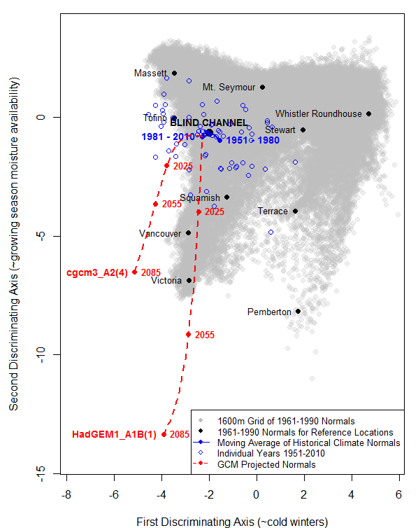
Projected climate changes for the next century appear to be much greater than the climatic variability at the regional scale. For this reason, climate change analysis and visualizations in climate space need to include climatic variation at the provincial or even continental scales. However, my investigation of climatic variation on the BC coast suggested that observed climatic variation at larger than regional scales is likely to be irregularly and/or non-linearly distributed in more than 3 dimensions of climate space. Dimension reduction using linear methods such as principal components analysis (PCA) or linear discriminant analysis (LDA) are fitted “globally” through the entire data, and are therefore likely to obscure dimensions of variation that are “locally” important to individual regions of the climate space and the landscape. This can inhibit visualizations of analogous and novel climatic conditions because conditions that are far apart in the full climate space may be close together in the reduced climate space. In contrast, many non-linear dimension reduction methods are able to combine uncorrelated locally important dimensions of variation onto a reduced global map of distance or similarity. Non-linear methods therefore offer a possible solution to the global vs. local dilemma.

General approaches to non-linear dimension reduction

There are many methods to reduce the dimensionality of non-linear data. A common approach is non-metric MDS, which is a category of methods that use iterative algorithms to find a low-dimensional arrangement of observations that best conserves some measure of distance or similarity between those observations in full-dimensional space. Neural networks have also been demonstrated as a robust approach for non-linear dimension reduction of climate data (Hsieh and Cannon 2008). Another general approach is to assume the data has “manifold structure”: that the data are arranged in a low-dimensional manifold that is embedded in high-dimensional space. A common analogy for manifold structure is a “jelly roll”, which is a rectangular plane embedded in three dimensions as a spiral. Many non-linear dimensionality reduction methods, including locally linear embedding (LLE) are designed to extract a low-dimensional manifold from a high-dimensional data space; in other words, to unroll the jelly roll.

Locally linear embedding

Locally linear embedding (Roweis and Saul 2000, Saul and Roweis 2003) is a prominent technique for nonlinear dimension reduction. Rather than attempt to find a global solution, this technique operates on local “neighbourhoods” within the data. LLE reconstructs data in lower dimensions by conserving the distances between each observation and a specified number of its nearest neighbours. LLE has been heavily modified and adapted to improve its performance for a variety of specialized purposes (e.g. (Ridder et al. 2003).

Experimental comparison of LLE with PCA and LDA

Simulation of Locally linear embedding compared to PCA and LDA

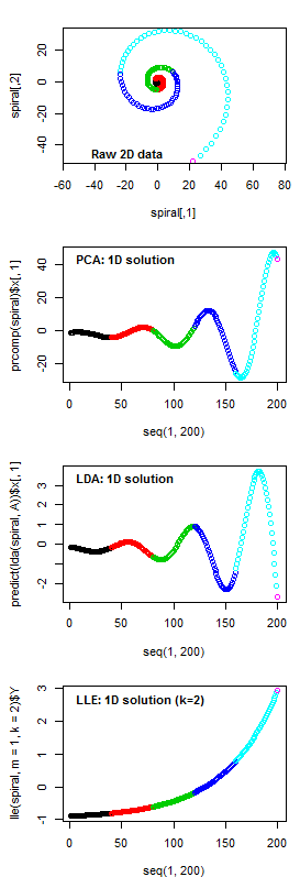
Figure 2: a comparison of dimension-reduction solutions provided by linear and non-linear methods. A two-dimensional logarithmic spiral is reduced to a one-dimensional index by Principal Components Analysis (PCA), Linear Discriminant Analysis (LDA), and Locally Linear Embedding (LLE), and plotted sequentially. Concept adapted from http://www.stat.cmu.edu/~cshalizi/350/lectures/14/lecture-14.pdf

Figure 2 illustrates the difference between LLE and both PCA and LDA (and between non-linear methods vs. linear methods more generally). A logarithmic spiral is inherently two-dimensional in a graphical sense, because it is the result of two out-of-phase oscillations with simultaneously increasing magnitude. However, spirals can also be viewed as a one-dimensional manifold imbedded in two-dimensional space. PCA and LDA can only provide axis rotations, and as a result, they can only capture one of the expanding oscillations, and do not provide a fundamentally different 1-dimensional solution than the first axis of the raw data for the spiral. LLE, in contrast, reduces the data to the distances between each point and its nearest neighbours (in this case, two of them), and reconstructs the spiral in one dimension based on these distances. In this way, LLE is successful in extracting the simple logarithmic relationship underlying both oscillations of the spiral. In other words, it is able to extract the one-dimensional manifold that was embedded in two dimensions as a spiral.

Is the non-linear LLE solution actually preferable for data visualization? From the perspective of classification, it is easy to see that LDA would be unable to effectively differentiate the colour-coded groups in one dimension. On the other hand, the LLE solution provides the basis for a perfect differentiation of groups. This advantage of LLE has been demonstrated on a variety of data sets (Ridder et al. 2003) and is a major reason why non-linear dimension-reduction methods such as LLE are preferred for artificial intelligence and other pattern recognition applications. However, LLE removed the oscillation from the signal, and so in a sense it produced a visualization that has no “spiralness.” While a spiral can be intuitively inferred from the PCA and LDA solutions, this inference is less obvious in the LLE solution. From a visualization perspective, the effectiveness of LLE over PCA is ambiguous.

Testing LLE on the climates of the BC coast

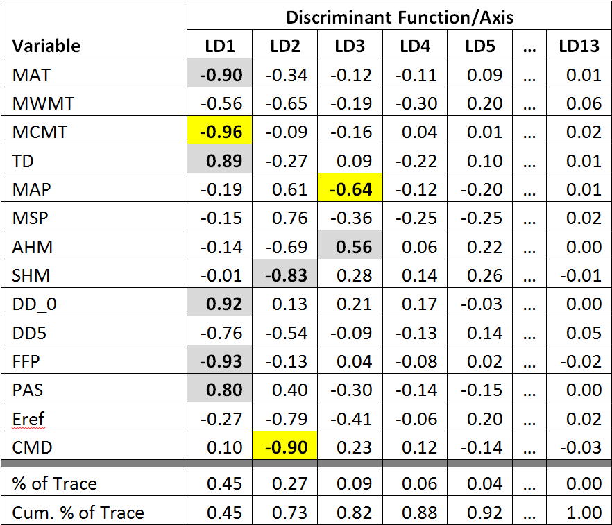
To test-run LLE on real climate data, LLE was used to produce a 3D reduction of 1961-1990 normals for the coastal British Columbia (BC). This is the same data used for discriminant analysis in the previous blog post. Input variables were MAT, MWMT, MCMT, TD, MAP, MSP, AHM, SHM, DD_0, DD5, FFP, and PAS. CMD and its precursor Eref were removed as input variables due to apparent problems with the calculation of CMD in ClimateWNA (I’ll save that for a future blog post). All variables were standardized by dividing by their standard deviation. Precipitation and heat-moisture variables (MAP, MSP, AHM, SHM, PAS) were log-transformed to normalize their distributions. PCA was done on these data using the “prcomp” call in the stats package of R. LLE was done using the “lle” call in the lle package of R. To test the effect of neighbourhood size on the solutions, four LLE runs were performed using k=3, 12, 48, and 200 nearest neighbours. LLE is very computationally intensive, and I had to reduce the data set by 8 (every eighth observation retained for analysis) in order to be able to run it on my laptop.

PC1 and PC2 of the PCA solution for the coastal data set

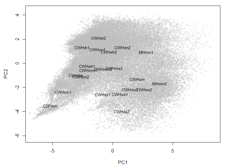
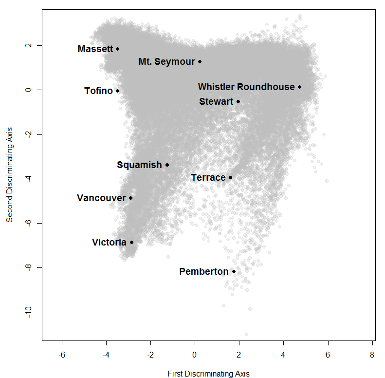
Figure 3: PCA dimension reduction solution for a 12-variable climate normal data set for the BC coast. The CWHwh1 and wh2 are incorrectly placed at the centre of the reduced climate space.

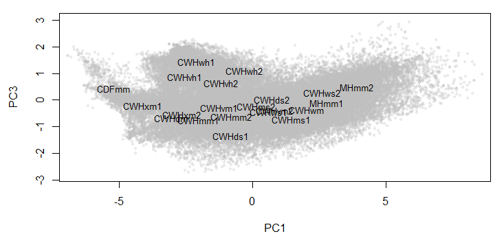
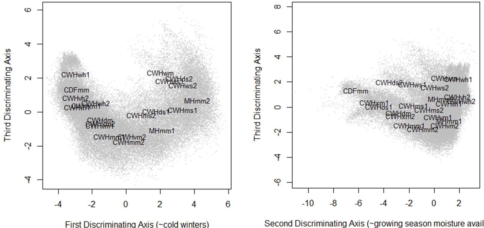
Figure 4: Third dimension of the PCA solution for the coastal data set, revealing that the CWHwh1 and wh2 are actually at one extreme of the full climate space.

The PCA solution for the coastal data set is shown in Figure 3 and Figure 4. The first three principal components represent 97% (58%, 33%, and 6%, respectively) of the variance in the data, which indicates that the data have an effective dimensionality of three despite being made up of 12 variables. PC1 and 2 provide a reasonable representation of the relationships between BEC variants, but incorrectly place the CWHwh1 and wh2 (Haida Gwaii) at the centre of the distribution. A third dimension (PC3) is required to correctly show that these variants are at one extreme of the distribution (Figure 4). The interactive 3D plot (Figure 5) shows that the normalized coastal data set has a dome-shaped distribution. This dome shape is a 2D manifold in 3 dimensions, plus noise. A successful non-linear solution would flatten this manifold into two dimensions and show the CWHwh1 and wh2 at the edge of the distribution. This criterion provides a means of evaluating how well LLE performs on real climate data.

Figure 5: 3D interactive plot of the LLE solution (use mouse to drag and zoom)

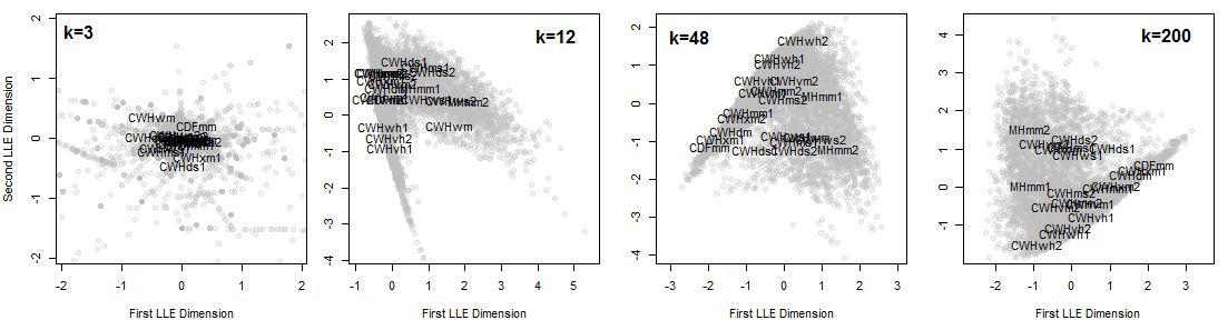
Figure 6: two-dimensional LLE dimension-reduction solutions for the coastal data set, using increasingly larger neighbourhoods (k=3, 12, 48, and 200 nearest neighbours).

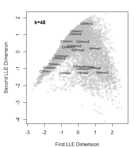
Figure 7: a closer look at the LLE solution using k=48 nearest neighbours.

The LLE solutions for the coastal data set are shown above. LLE on small neighbourhoods (k=3, k=12) did not provide stable or meaningful solutions (Figure 6). Large neighbourhoods (k=48, k=200) produced functionally equivalent solutions. The k=48 solution (Figure 7) exhibits the desired behaviour of placing the CWHwh1 and wh2 at one extreme of the distribution while maintaining the CDFmm and the MHmm2 at opposite extremes. The

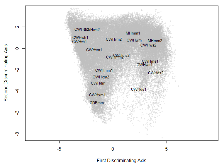
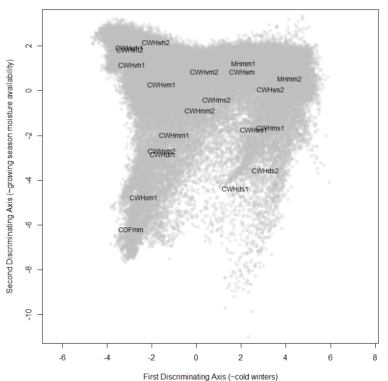
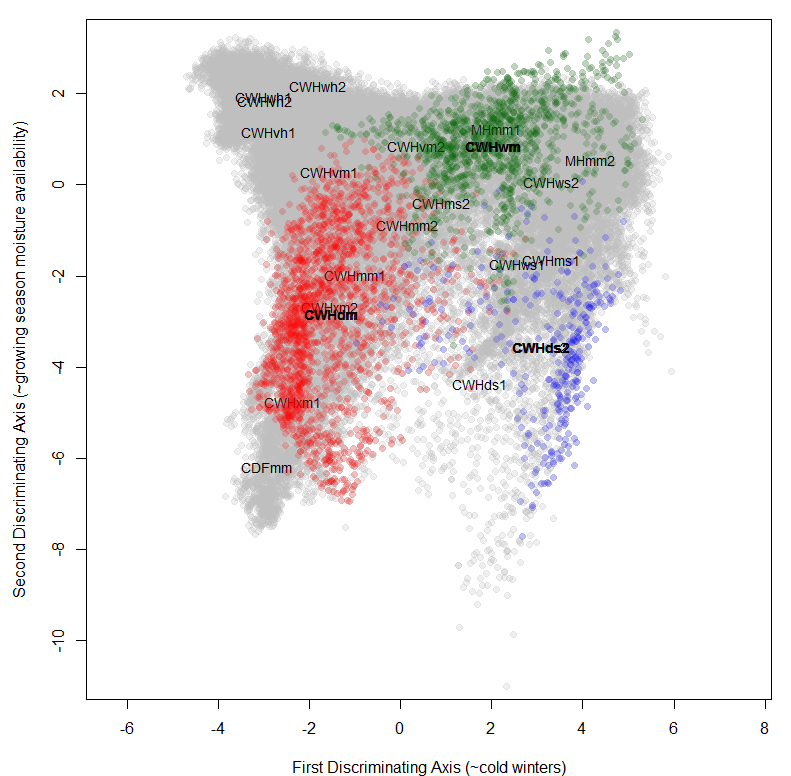
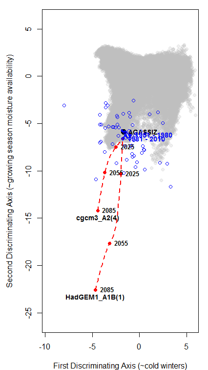
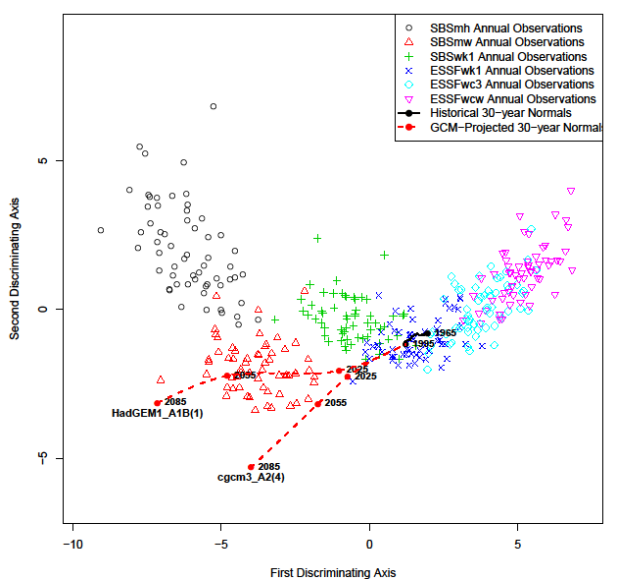
Figure 8: LDA solution for the coastal data set.

rank positions of the other BEC variants also make sense for the most part, although the relative proximity of the CWHds2 to the MHmm2 is problematic. Despite these apparent successes, the distribution of observations appears compressed towards the hypermaritime variants. Similar distortions appear to be common with LLE, even in showcased solutions on idealized data sets (e.g. Saul and Roweis 2003). This compression is extremely problematic for climate change visualization, because the magnitude of change will be exaggerated in some areas of the reduced climate space, and diminished in others. In comparison to an LDA solution (Figure 8), the LLE solution is not as satisfying.

Discussion

The goal of LLE and many other non-linear dimension reduction methods is to reduce manifold structures down to the intrinsic dimensionality of the manifold itself, i.e. to “unroll the jelly roll”. It is likely that climate data have a roughly manifold structure, because the observations are taken across a two-dimensional geographic surface and thus the distribution in climate space is likely to be constrained. However, the usage of LLE and other manifold learning algorithms for multivariate climate surfaces doesn’t appear to have been validated in the literature. Even if climate surfaces have a non-linear manifold structure (e.g. the dome shape evident in the three-dimensional PCA and LDA solutions for coastal BEC variants), that structure may have important climatic and ecological meaning. It means that some climate variables are important in some areas of climate space but not in others. As with the spiral experiment, linear methods will preserve non-linear relationships in the data space, and this may be a desirable result for visualization at regional and subregional scales.

LLE results are likely to be much more difficult to interpret in terms of the original input variables. LLE dimensions can be correlated with the raw variables of the full data space. However, these correlations could potentially have large variations across the distribution of data in the reduced data space. Also, it would be entirely possible for one LLE dimension to be correlated with two entirely uncorrelated climate variables. As a result, interpretations of the climatic meanings of the LLE dimensions would be unreliable, notwithstanding measures such as correlation mapping across the reduced climate space.

From a practical perspective, my project requires the ability to project new data into the reduced climate space. It is unclear whether it would be possible to map new data in an LLE-reduced data space. However, mapping of new data is feasible in other non-linear methods (Hsieh and Cannon 2008). Another essential practical consideration is that the computational requirements of LLE are prohibitive at anything larger than the regional scale. My computer could not run LLE on more than 10,000 observations, even using small neighbourhoods (k<12). This limitation makes LLE unfeasible for everyday use.

Despite these potential pitfalls, non-linear methods such as LLE have the potential to map the distances between observations regardless of the dimensions in which those distances occur. This is potentially a very useful feature for visualizing the magnitude of climate change, even if it obscures the climate variables in which those changes are occurring. Non-linear dimension reduction methods should be further evaluated, alongside mainstream linear methods.

Conclusion

The strength of non-linear approaches in theory is that they have the potential to map the distances between observations regardless of the dimensions in which those distances occur. In theory, this could produce multivariate data mappings at lower dimensionality than would be possible with linear methods. This is potentially very important for climate change visualization at provincial or continental scales, where there are likely to be many more than three important dimensions of climatic variation. The two analyses presented here confirm that LLE is able to extract a lower-dimensional manifold from higher-dimensional data, even on real, noisy climate data. However, LLE appeared to create non-linear distortions in the reduced data space, which is a severe drawback for climate change visualization. In addition, interpretation of LLE dimensions is confounded because they can be made up of uncorrelated variables. Finally, LLE is extremely computationally intensive. Non-linear dimension reduction approaches deserve further investigation due to their theoretical advantages, but this case study of LLE suggests that the search for an appropriate method may be very time-consuming. Linear methods such as LDA and PCA appear to be adequate at the regional scale. For the moment, I will focus on my immediate research objectives, and return to non-linear methods at a later date.

References

Hsieh, W. W., and A. J. Cannon. 2008. Towards Robust Nonlinear Multivariate Analysis by Neural Network Methods. Lecture Notes in Earth Sciences 112:97–124.

Ridder, D. De, O. Kouropteva, O. Okun, M. Pietikainen, and R. P. W. Duin. 2003. Supervised locally linear embedding. Pages 333–341, Artificial Neural Networks and Neural Information Processing — ICANN/ICONIP 2003.

Roweis, S. T., and L. K. Saul. 2000. Nonlinear dimensionality reduction by locally linear embedding. Science 290:2323–6.

Saul, L. K., and S. T. Roweis. 2003. Think Globally , Fit Locally : Unsupervised Learning of Low Dimensional Manifolds 4:119–155.

Discriminant analysis of climatic variation and change across coastal British Columbia

Leave a reply

The Seasons Alter: Climate Change at Blind Channel, BC

Visualization of historical and projected future climate change at Blind Channel, BC.

Summary

This blog post is a test run of a linear discriminant analysis (LDA) method for climate change visualization. The objective of this analysis is to create a low-dimensional (2D or 3D) climate space that reasonably represents the geographic variation of climate on the BC coast, and use that climate space to contextualize historical climatic variability and projected climate changes at selected locations. The analysis produced following outcomes:

LDA appears to have produced a meaningful reduced climate space that reasonably represents the relationships between BEC variants. The regional scale appears to be more appropriate than the local (transect) or provincial scale;
The backdrop of regional climatic variation provided a useful context for historical interannual climate variability and projected climate changes. However, projections into regionally novel climate space were difficult to evaluate due to absence of potential climatic analogs from outside the region;
There appear to be dramatic sub-regional differences in the scale and novelty of projected climate change. Climate change on the north coast appears to be relatively moderate, and stays within the existing range of regional variation. In contrast, climate change on the south coast appears to be of much greater magnitude and entirely into regionally novel conditions.

The key next steps are to develop and test-run other alternative dimension-reduction methods such as multidimensional scaling, and to develop methods to visualize distant climatic analogs and truly novel climate space.

Introduction

In a previous blog post I discussed the results of a discriminant analysis of BEC variants along an elevational transect in central interior of BC. My conclusion was that only the first discriminant axis was meaningful. The other axes represented non-linearities in the relationships between the climatic variables, and did not have an intuitive climatic interpretation. As a result, discriminant analysis, though useful for classification, is likely of dubious value as a method for creating low-dimensional climate visualizations in a simple climatic gradient. Nevertheless, I was curious how discriminant analysis performs on a larger and more complex climatic landscape. It is possible that meaningful variation in the second and third dimensions will relegate problematic non-linearities to lesser dimensions.

The purpose of this blog post is to test run an LDA-driven climate change visualization at a regional scale. I do a discriminant analysis on the 1961-1990 climate normals over a 1600-metre grid of coastal British Columbia. The results are evaluated in 2D and 3D climate space. Then I plot historical interannual variability and projected climate change for individual locations to get a glimpse of what climate change visualizations might look like in the reduced climate space.

Biogeoclimatic Climate Classification for the Coast

The coastal region provides a good case study because it has a relatively simple climatic geography, compared to the interior of BC. The climatic variation of the coast can be understood in a simple sense in terms of four climatic gradients:

dry in the south vs. wet in the north, due to the influence of the Aleutian low;
wet belts and rainshadows associated with the mountains of Vancouver island, the Olympic Peninsula, Haida Gwaii, and the Coast Range;
hypermaritime (low seasonality of temperature) on the outer coast vs. submaritime (hot summers, cold winters) inland, due to the moderating influence of the Pacific Ocean; and
Decreasing annual temperatures with elevation.

The Seasons Alter: Vancouver BEC Variants

Figure 1: An example of the BEC climate classification: BEC variants of Vancouver BC.

The Biogeoclimatic Ecosystem Classification (BEC) includes a detailed classification of the climates of the coast. The naming conventions of the BEC climate classification of are simple to understand and worth knowing. The vast majority of the coast is classified as the Coastal Western Hemlock Biogeoclimatic Zone. The exceptions are the Coastal Douglas-Fir (CDF) zone in the mediterranean climate of the Georgia Basin, and the Mountain Hemlock (MH) zone in subalpine elevations. Subzones are named with a two-letter code corresponding to their relative precipitation (x=very dry, d=dry, m=moist, w=wet, v=very wet) and continentality (h=hypermaritime, m=maritime, s=submaritime). Each subzone generally has at least two variants. In the CWH, variants are either elevational (1=submontane, 2=montane; CWHmm/vm/wh/ws) or latitudinal (1=southern, 2=central; CWHds/ms/vh). In the MH zone, variants are windward (1) vs. leeward (2). Figure 1 shows a small portion of the BEC variant mapping of the coast to provide a sense of the scale of the BEC climate classification.

Methods

Observations are locations on a 1600-m grid clipped to the geographic range of the CWH, CDF, and MH zones (MHmm1/2 only). I used the following annual climate normals output from ClimateWNA: MAT, MWMT, MCMT, TD, MAP, MSP, AHM, SHM, DD_0, DD5, FFP, PAS, Eref, and CMD. I log-transformed precipitation and heat-moisture variables (MAP, MSP, AHM, SHM, PAS) to normalize their distributions. LDA was done on these data using the “lda” call in the MASS package of R.

Results

The Seasons Alter: Table 1: Correlation structure of the LDA

Table 1: Correlations between climate variables and the first 5 of 13 linear discriminant functions. Primary correlations are highlighted grey, and the leading correlation is highlighted yellow. “% of trace” is an unrelated index of the percent of between-class variation explained by each discriminant function.

The structure of the LDA is strikingly different from that of the Quesnel-Barkerville transect. The first three discriminant functions (LD1-3) explain a moderate 82% of the between group variance of the coastal BEC variants (bottom of Table 1), which was the same amount explained by LD1 alone in the Quesnel-Barkerville transect. This is no doubt because the coastal region contains many climatic gradients, rather than just one. The correlations between the major discriminant axes (Table 1) are also more easily interpretable than in the transect analysis. LD1 appears to be an index of cold winters, and LD2 appears to be an index of growing season moisture availability (i.e. a negative drought index). LD3 appears to be a negative index of precipitation, especially of winter precipitation.

2D visualization of the coastal climate space

The Seasons Alter: Simplified LDA plot with BEC variant labels

Figure 2: Simplified plot of the coastal grid in the first two discriminant axes, with BEC variants labelled at their climatic centroids.

Figure 3: ClimateBC normals for some reference locations

The relative positions of the BEC variants in the first two dimensions make sense in the context of these climatic indices (Figure 2). The progression from the bottom left to top right (CDFmm to MHmm1) is essentially the sequence of BEC variants moving outwards from the Georgia basin and upwards into the mountains of Vancouver Island and the coast range. The progression from the bottom right to the top left (CWHds1 to wh1) is the sequence of BEC variants from the coast-interior transition zone to the outer coast. The gap between the maritime and submaritime BEC variants in the first dimension is likely due to the presence of the coast mountains; i.e. the narrow glacial valleys connecting these two groups do not contribute enough grid points to fill the transition. The only pairing of BEC variants that doesn’t make sense in the first two dimensions is the CWHwm (sea level) and MHmm1 (subalpine). Overall, this appears to be a valid low-dimensional representation of the coastal climate space.

Figure 4: Grid points in the third discriminating axis plotted against the first and second axes.

The third dimension of the coastal discriminant climate space is shown two-dimensionally in Figure 4, and below as an interactive three-dimensional visualization. There is a pronounced three-pointed arch shape in the third dimension. However, it is not clear whether this is a cryptic artifact of non-linearities in the data, or a meaningful climatic phenomenon. The correlation structure of the LDA (Table 1) suggests that the third axis is an index of winter dryness. The plot of the second and third dimensions (Figure 4, right) clearly distinguishes the rainshadows of the Olympic Peninsula/Vancouver Island (CDFmm), the Coast Range (CWHds2/ws1), and Haida Gwaii (CWHwh1). Interestingly, the CWHvh1 and vh2 also have intermediate values in the third dimension. This result makes sense, despite the common misconception that the hypermaritime subzones experience the highest rainfall on the coast; large areas of the CWHvh1 and vh2 are outer coastal lowlands that experience more summer fog than adjacent maritime subzones (e.g. CWHvm1) but less frontal precipitation due to the lack of orographic uplift. The CWHwm and MHmm1, which were poorly discriminated in the first two dimensions, are well discriminated in the third dimension. Despite the consistency of these observations with patterns of winter precipitation, the arch-shaped relationship between the first and third dimensions is questionable. It would take further investigation to determine whether this relationship is cryptic or meaningful. For this reason, I use only the first two dimensions for the remainder of the analysis.

Interactive 3D visualization (drag and zoom to explore the climate space)

Distribution and overlap of BEC variants within the climate space

The Seasons Alter: Table 2: Classification error

Table 2: Classification error rates of the discriminant analysis, indicating the number of grid cells that fell within another BEC variant’s domain in full-dimensional climate space. Prior probabilities are simply the proportion of the total number of 1600-m grid cells in each BEC variant.

Figure 6 shows the distribution of grid point normals for three arbitrarily selected BEC variants. The grid points of each BEC variant are disperse widely through the first two dimensions, and overlap with numberous BEC variant centroids. Superficially, this suggests low accuracy of the BEC variant mapping and/or of the ClimateWNA/PRISM data. However, the classification error of the discriminant analysis is 37% (Table 2). This indicates that almost 63% of the area of the BEC variants fall into their own exclusive region of the full-dimensional climate space. The remaining 37% classification error is a combination of errors in the BEC variant mapping, ClimateWNA/PRISM surfaces, and variable selection, in unknown proportions. These results indicate that ClimateWNA data can reasonably differentiate BEC variants in full-dimensional climate space, but that differentiation in low dimensional climate space is poor. The climatic centroid of BEC variants is likely much more meaningful in reduced dimensions than the boundaries between BEC variants.

Figure 5: Spatial variability of ClimateBC output for three BEC variants.

Visualizing historical and projected climate change in the 2D discriminant climate space

Figure 6: locations of the weather stations used for the climate change visualizations. The distribution of the Coastal BEC zones is shown in green.

The locations of three long-term weather stations were selected as case studies for climate change visualization (Figure 6). These sites roughly represent the northern, central, and southern regions of the BC coast, though Blind Channel is in an area that is climatically transitional between the southern and central regions. Although these are weather station locations, it is important to note that all date presented here is from ClimateWNA.

The graph for Stewart (Figure 7) can be used to introduce the elements of the climate change visualizations. The case study location is labeled at the position of the 1961-1990 normals in climate space. The climatic conditions of individual years in the period 1951-2010 at the case study location are shown as empty blue circles. A 30-year moving average of these years, shown as a blue line, shows the drift in climate normals starting with the 1951-1980 normals, and ending with the 1981-2010 normals. Future climate normals projected by two GCMs are shown as red dots and labelled by median year. The red dotted line is a spline interpolation with no climatic meaning except to visually connect the projected normals. Collectively, the intent of all these graphic elements is to contextualize GCM projections in terms of historical climatic variability and regional climatic variation.

Climate change visualization for Stewart, BC

Figure 7: Historical climatic variability and GCM-projected climate change at Stewart, BC.

Stewart visualization in the third dimension

Figure 8: GCM projections for Stewart BC in the third discriminant dimension

Historical interannual climatic variability at Stewart is substantial, though the range of variability generally falls within the 2D climate envelope of the coast. Despite this interannual variability, climate change has been limited over the past 60 years at Stewart, as suggested by the blue moving average of climatic normals. Nevertheless, there is a trend towards droughtier conditions. Neither of the GCM runs project a continuation of drying trend in the 2011-2040 normal period (labelled “2025”). Instead, they both project a moderate to rapid shift towards warmer winters initially, then a shift towards warmer winters and droughtier growing seasons. Within the 2D climate space, there are historical climatic analogs for the end point of both projections: conditions in the 2071-2100 normal period (labeled “2085”) are similar to the 1961-1990 climate normals for Agassiz the HadGEM1_A1B(1) run and for Port Renfrew in the cgcm3_A2(4) run. These analogs also apply in the third dimension (Figure 8).

Climate change visualization for Blind Channel

Figure 9: Historical climatic variability and GCM-projected climate change at Blind Channel, BC.

The other two case studies are more than 5 degrees of latitude south of Stewart, and in the neighbouring GCM grid cell. Projected climate changes in these two case studies are more dramatic, especially at Agassiz. The endpoint of both GCM runs is entirely novel to the coast, and well beyond the range of interannual variability over the past 60 years. It is worth noting here that a climate envelope classification based on discriminant analysis would likely classify these novel endpoints as CDFmm due to the lack of available analogs.

climate change visualization for Agassiz, BC

Figure 10: Historical climatic variability and GCM-projected climate change at Agassiz, BC.

The most striking pattern of the three case studies is that the apparent scale of climate change is dramatically greater in the south coast. Whether or not this reflects the relative scales of climate change in the GCM runs is yet to be investigated. The most likely reason for this effect is that the second discriminating axis exaggerates changes towards progressively drier conditions. This is entirely possible because CMD was not log-transformed even though it is partially derived from precipitation. To check this hypothesis, I reran the analysis without CMD and Eref. Surprisingly, the results were very similar. Further investigation is required to determine whether the second axis contains distortions that exaggerate climate change in drier areas of the climate space.

Overall evaluation of the method

The purpose of this analysis was to create a low-dimensional (2D or 3D) climate space that reasonably represents the geographic variation of climate on the BC coast, and use that climate space to historical climatic variability and project climate changes. Was the method successful? Here are my thoughts:

Discriminant analysis of the 1961-1990 normals of the 1600m grid locations produce a 2D climate space that reasonably represents the relationships between BEC variants, with some exceptions. These exceptions were resolved in the 3D climate space. It is likely that this reduced climate space could be improved through careful variable selection and transformation. Notably, CMD is calculated from climate normals in ClimateWNA, which skews its distribution towards zero. For this reason, CMD (and its precursor Eref) should be either dropped from the analysis or recalculated from monthly observations.
The dimensions of the reduced climate space for the coast are climatically meaningful, and are relatively free of the cryptic artefacts that drove the second and third dimensions of the Quesnel-Barkerville transect. This indicates that there is a “goldilocks”-type sweet spot for the scale of study areas for reduced climate spaces. Transects are too small, because they only represent a single axis of climatic variation. The province is too big, because it contains many important axes of variation that cannot be meaningfully represented in 2D or 3D. The regional scale appears to be “just right”. Of course, it is unclear whether the “novel conditions” portrayed in the case studies are truly novel or just regionally novel. This is the tradeoff between local vs. global classification that I discussed in the previous blog post. Nevertheless, it may be possible to resolve this tradeoff with the right method.
This background of regional variation provides a useful context for interannual variability and climate change. However, the (possibly fatal) flaw of this approach is that it constrains the representation of climate variability and change to the primary dimensions of existing geographic variation (winter temperature and summer drought in this case). Variation in other dimensions is invisible, even though it may be highly biologically relevant. This is a potential problem in situations like the visualization for Stewart, where there appeared to be climatic analogs for the projections in 2D and 3D space. It is much less of a problem where novel conditions are projected in 2D, as in Blind Channel and Agassiz, since it is highly unlikely that analogs would exist in full-dimensional climate space that don’t exist in the reduced space.
Projections of climate change into novel areas of the climate space are visually dramatic. However, the discriminant axes may conceal non-linearities that distort the representations of these changes. Any axes created through discriminant analysis require extensive validation.
This analysis was primarily an exercise in visualization. In order for the method to be successful, however, it must also facilitate quantitative analyses of climatic variability, differentiation, and novelty. I’m not yet convinced that discriminant analysis provides reliable axes (metrics) for quantitative purposes.

Next steps

Develop and test-run some other methods for achieving the same objective. The most obvious alternate approach is multidimensional scaling. Another alternate approach is to use LDA or some other method to assist with supervised variable selection, and use raw climatic variables as visualization axes. For example, it appears from this analysis that MCMT, SHM, and MAP may be viable first, second, and third axes for a more intuitive reduced climate space for the coast region. Ultimately, the method must be compatible with a quantitative analysis of climatic variability, differentiation, and novelty (a la Williams et al. 2007).
Develop methods to resolve the compromise between local and global classifications. An example of a potential approach is a two-step graphical approach. The first graph would plot grid points for the entire western North America in the discriminant axes of the coastal climate space and portray GCM projections for a focal (BC coastal) location against this background. The axes of the second graph could be the discriminant axes for the climatic analog (Oregon? California?) for the projected conditions of the focal location. This approach would provide a graphical validation of the inferred analog. Localized LDA (described in the previous blog post) may be a viable method for this approach.
Evaluate the pros and cons of including interannual climatic variability and the GCM projections into the discriminant (or alternate) analysis. The advantage would be that the reduced climate space could portray key axes of temporal variability that don’t exist in the geographic climatic variation. The disadvantage is that it may be difficult to simultaneously represent spatial and temporal variability in a reduced climate space at the regional scale. This approach may only be viable for transects.

References

Williams, J. W., S. T. Jackson, and J. E. Kutzbach. 2007. Projected distributions of novel and disappearing climates by 2100 AD. Proceedings of the National Academy of Sciences of the United States of America 104:5738–42.

Global vs. localized linear discriminant analysis for understanding climatic differences between BEC variants

Leave a reply

Linear Discriminant analysis (LDA) is an attractive means of comparing BEC variants in a reduced climate space because it emphasizes the climate variables that differentiate BEC variants. However, it is essential to note that LDA is a global classifier: the models (linear discriminating functions) maximize the ratio of total between-group to within-group variance across all groups. This “one size fits all” approach is appropriate where the processes (variables) generating the differences between groups are reasonably consistent across all groups. However, poor model fit in a reduced climate space is expected if the discriminating processes differ in various regions of the data space. This is certainly the case with the BEC climate classification.

The beauty of the BEC climate classification is that rather than defining climates in terms of predefined quantitative climate variables, it infers climate differences based on differences in vegetation communities. The climate variables creating these vegetation differences are expected to be different for each pair of adjacent BEC variants. In some cases, snow depth may be the crucial variable, in others it may be growing season frost, drought, and so on. LDA on the entire province cannot be expected to capture the important differences between BEC variants. It is likely that any LDA solution at the provincial or even regional level will be overly reductive. There appears to be a tension between the need to represent local differences accurately and the need to understand the system as a whole. It would be desirable to have a methodology that was able to integrate a localized analysis of the differences between adjacent pairs of BEC variants with a provincial scale analysis.

Czogiel et al. (2007) provide a very nice summary of the issue:

Since the estimation is carried out without taking into account the nature of the problem at hand, i.e. the classification of a specific trial point, LDA can be considered a global classifier. Hand and Vinciotti (2003) argue that an approach like this can lead to poor results if the chosen model does not exactly reflect the underlying data generating process because then, a good fit in some parts of the data space may worsen the fit in other regions. Since in classification problems accuracy is often not equally important throughout the entire data space, they suggest to improve the fit in regions where a good fit is crucial for obtaining satisfactory results – even if the fit elsewhere is degraded. For the dichotomous logistic discrimination, two approaches have been proposed to accomplish this. Hand and Vinciotti (2003) introduce a logistic discrimination model in which data points in the vicinity of the ideal decision surface are weighted more heavily than those which are far away. Another strategy is presented by Tutz and Binder (2005) who suggest to assign locally adaptive weights to each observation of the training set. By choosing the weights as decreasing in the (Euclidian) distance to the observation to be classified and maximizing the corresponding weighted (log-)likelihood, a localized version of the logistic discrimination model can be obtained. The classifier is therefore adapted to the nature of each individual trial point which turns the global technique of logistic discrimination into an observation specific approach.

Czogiel et al. (2007) go on to describe a method they call “localized linear discriminant analysis”. This approach modifies LDA using locally adaptive weights. They state that this is a simpler approach than earlier approaches (e.g. Hand and Vinciotti 2003) based on logistic discrimination. It also is usable with multi-class situations, which logistic discrimination is not.

The introduction is compelling, but they did not provide a plain-language description of their method, and the mathematical description of their approach was over my head. The examples they provided were also not very instructive for me.

However, the basic concept appears to be relevant to the problem of fitting multi-class LDA models to local conditions. Rather than treating several BEC variants (or several hundred, as in the case of a BC-scale analysis) as equal, it might be possible to use an approach that puts a single location at the centre of the climate space classification. Instead of asking “what do BEC variants look like in climate space?”, we would be asking “what does climate space look like from the perspective of the ESSFwk1?” discrimination (maximizing the ratio of between-group variance to within-group variance) could be weighted based on Euclidian distance of group centroids. This would favour discriminating functions that emphasize the variables responsible for differentiation of the neighbours of the focal variant in climate space.

What would this approach achieve?

1. For each BEC variant, there would be an ordered list of which climate variables differentiated it from its neighbours in climate space. This is interesting from an ecological perspective.

2. This approach would customize dimension reduction for the climatic context of an individual location. This would likely be a preferable climate space for visualizing historical and projected climate change at that location. By changing the weighting function, the realm of the climate space could be expanded or contracted as needed to incorporate large projected climate changes.

Localized LDA is an intriguing idea. It may suffer from the same flaws as discriminant analysis on an environmental gradient. On the other hand these flaws may be partially mitigated by the presence of the full set of 200+ BEC variants being available. While not as straightforward and promising as multidimensional scaling, localized LDA is worth considering as an option for analysis and visualization of climate change relative to the BEC climate classification.

References

Czogiel, I., K. Luebke, M. Zentgraf, and C. Weihs. 2007. Localized linear discriminant analysis. Pages 133–140 in R. Decker and H. Lenz, editors. 30th Annual Conference of the German-Classification-Society.

Hand, D. J., and V. Vinciotti. 2003. Local Versus Global Models for Classification Problems. The American Statistician 57:124–131.

A brainstorm of methods for creating low-dimensional climate spaces for climate change visualization

Leave a reply

One of my early attempts at visualizing historical and projected climate change.

Visualization of climate change is an important objective of my research. Without good visualizations, it is unlikely that my results will have much impact on even the most technical audience. However, portraying climatic variability and change in 2- or 3-dimensional space is extremely difficult without oversimplifying or abstracting the results. Trying visualize the “truth” of climate change in two or three dimensions may turn out to be in the same camp as searching for the holy grail, cold fusion, and perpetual motion… but I can’t resist giving it a decent try.

The previous blog found that discriminant analysis on the Quesnel-Barkerville BEC variants did not produce a meaningful visualization of climate space. The objective of the discriminant analysis in this case was to provide a reduced climate space in which trajectories, velocity, and novelty of climate change can be visualized relative to the differentiation between BEC variants. The first discriminant axis provided a meaningful index of dry/warm conditions. However, the second and third axes did not have an intuitive climatic interpretation. Importantly, the ability to detect novel conditions was likely severely constrained, because the dry/moist axis that inherently existed in the full-dimensional climate space was essentially removed from the reduced 5-dimensional discriminant climate space. These are fatal flaws for the use of discriminant analysis for the stated objective. It is very likely that other variance-based approaches (e.g. principle components analysis) would suffer from similar problems.

Despite these problems, I am not ready to abandon discriminant analysis entirely. It has the very desirable benefit of finding a low number of dimensions that efficiently define the differences between BEC variants. In the case of the Quesnel-Barkerville BEC variants, 79% of the total discrimination achieved by the analysis, following log transformations, occurred in the first dimension (if I am interpreting the meaning of “proportion of trace” correctly). It is possible that with further judicious transformations the discriminating power of the first dimension could be increased even further. In other words, discriminant analysis provided a single axis that described the essential differences between the six BEC variants. The problem with the analysis was in the second and third axes. The first axis is the baby; the second and third axes appear to be the bathwater.

One possible solution would be to find a second and third axis that describe climatically meaningful orthogonals to the first discriminating axis. The first axis in the Quesnel-Barkerville analysis appears to be an index of dry/warm. The second axis could be an orthogonal wet/warm index. This could be done in three dimensions too if a third component was apparent in the axis1 index (e.g. snow depth, continentality). I’m not sure what the criteria would be to choose the orthogonals, but the idea is worth some further thought.

That’s one idea, but I obviously need to do a review of my options. The following is a brainstorm of potential approaches that need some research and/or consideration:

Modifications of LDA, as described above.
Multidimensional Scaling (MDS). This is a broad class of techniques for dimension reduction. The common goal of MDS techniques is to preserve between-object distances as well as possible in a predetermined subset of dimensions.
Supervised variable selection. This approach would use raw (unrotated) variables as axes for a 2- or 3-dimensional simplified climate space. In other words, this is feature selection rather than the feature extraction performed by axis rotation (e.g. LDA, PCA). The key would be to choose a single focal BEC variant and select 2 or 3 variables that most powerfully differentiate the focal BEC variant from its neighbours in high-dimensional climate space. This focal-variant approach is viable because climate change trajectories are visualized for individual geographical locations. the analysis could be iterated through raster cells for regional/provincial scale summaries and maps.
Localized linear discriminant analysis (Czogiel et al. 2007). This approach is similar to raw variable selection for focal variants, but it does a localized feature extraction (LDA) instead. Rather than treating all groups as equal for calculation of the discriminating functions, this approach weights the calculation based on proximity of each group to a single multivariate coordinate (e.g. the climatic centroid of a BEC variant). This approach seems to be pretty obscure, but it is worth investigating.
Exotic visualization techniques, e.g. Information Flocking Boids. There are a lot of attractive but mathematically opaque approaches out there. While these are worth a cursory review, I have a feeling I could go down the rabbit hole with this stuff.
No dimension reduction: just use measures such as Standardized Euclidian distance (Williams et al. 2007) or clustering to describe shifts into analogous or non-analogous climate space. Results can be visualized by mapping them geographically (e.g. colour coding raster cells by degrees of climatic novelty). While a full-dimensional analysis is likely an important component of my research, I am reluctant to give up on portraying visualizations of climate change in reduced climate space.

I will evaluate each of these approaches in future blog posts.

References