Summary
This blog post investigates locally linear embedding (LLE), a prominent and heavily-adapted technique for non-linear dimension reduction. The strength of non-linear approaches in theory is that they can map distances in climate space at a much lower dimensionality than linear methods. First, a simple experimental data set is used to compare LLE to principal components analysis (PCA) and linear discriminant analysis (LDA). Second, an LLE-reduced climate space for the BC coast is compared to the PCA and LDA climate space. The two analyses did not show clear advantages of LLE over the linear methods at the regional level, despite some promising results. More generally, it appears that finding and validating a reliable non-linear dimension reduction method is likely to be time-consuming and beyond the scope of my project at this point. Nevertheless, the potential for non-linear methods to solve the “global vs. local” dimension reduction dilemma cannot be ignored. It is likely that I will return to non-linear methods at a later date.
Introduction: non-linear methods as a potential solution to the “global vs. local” dimension reduction dilemma.
Projected climate changes for the next century appear to be much greater than the climatic variability at the regional scale. For this reason, climate change analysis and visualizations in climate space need to include climatic variation at the provincial or even continental scales. However, my investigation of climatic variation on the BC coast suggested that observed climatic variation at larger than regional scales is likely to be irregularly and/or non-linearly distributed in more than 3 dimensions of climate space. Dimension reduction using linear methods such as principal components analysis (PCA) or linear discriminant analysis (LDA) are fitted “globally” through the entire data, and are therefore likely to obscure dimensions of variation that are “locally” important to individual regions of the climate space and the landscape. This can inhibit visualizations of analogous and novel climatic conditions because conditions that are far apart in the full climate space may be close together in the reduced climate space. In contrast, many non-linear dimension reduction methods are able to combine uncorrelated locally important dimensions of variation onto a reduced global map of distance or similarity. Non-linear methods therefore offer a possible solution to the global vs. local dilemma.
General approaches to non-linear dimension reduction
There are many methods to reduce the dimensionality of non-linear data. A common approach is non-metric MDS, which is a category of methods that use iterative algorithms to find a low-dimensional arrangement of observations that best conserves some measure of distance or similarity between those observations in full-dimensional space. Neural networks have also been demonstrated as a robust approach for non-linear dimension reduction of climate data (Hsieh and Cannon 2008). Another general approach is to assume the data has “manifold structure”: that the data are arranged in a low-dimensional manifold that is embedded in high-dimensional space. A common analogy for manifold structure is a “jelly roll”, which is a rectangular plane embedded in three dimensions as a spiral. Many non-linear dimensionality reduction methods, including locally linear embedding (LLE) are designed to extract a low-dimensional manifold from a high-dimensional data space; in other words, to unroll the jelly roll.
Locally linear embedding
Locally linear embedding (Roweis and Saul 2000, Saul and Roweis 2003) is a prominent technique for nonlinear dimension reduction. Rather than attempt to find a global solution, this technique operates on local “neighbourhoods” within the data. LLE reconstructs data in lower dimensions by conserving the distances between each observation and a specified number of its nearest neighbours. LLE has been heavily modified and adapted to improve its performance for a variety of specialized purposes (e.g. (Ridder et al. 2003).
Experimental comparison of LLE with PCA and LDA
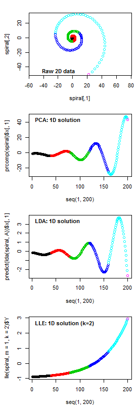
Figure 2: a comparison of dimension-reduction solutions provided by linear and non-linear methods. A two-dimensional logarithmic spiral is reduced to a one-dimensional index by Principal Components Analysis (PCA), Linear Discriminant Analysis (LDA), and Locally Linear Embedding (LLE), and plotted sequentially. Concept adapted from http://www.stat.cmu.edu/~cshalizi/350/lectures/14/lecture-14.pdf
Figure 2 illustrates the difference between LLE and both PCA and LDA (and between non-linear methods vs. linear methods more generally). A logarithmic spiral is inherently two-dimensional in a graphical sense, because it is the result of two out-of-phase oscillations with simultaneously increasing magnitude. However, spirals can also be viewed as a one-dimensional manifold imbedded in two-dimensional space. PCA and LDA can only provide axis rotations, and as a result, they can only capture one of the expanding oscillations, and do not provide a fundamentally different 1-dimensional solution than the first axis of the raw data for the spiral. LLE, in contrast, reduces the data to the distances between each point and its nearest neighbours (in this case, two of them), and reconstructs the spiral in one dimension based on these distances. In this way, LLE is successful in extracting the simple logarithmic relationship underlying both oscillations of the spiral. In other words, it is able to extract the one-dimensional manifold that was embedded in two dimensions as a spiral.
Is the non-linear LLE solution actually preferable for data visualization? From the perspective of classification, it is easy to see that LDA would be unable to effectively differentiate the colour-coded groups in one dimension. On the other hand, the LLE solution provides the basis for a perfect differentiation of groups. This advantage of LLE has been demonstrated on a variety of data sets (Ridder et al. 2003) and is a major reason why non-linear dimension-reduction methods such as LLE are preferred for artificial intelligence and other pattern recognition applications. However, LLE removed the oscillation from the signal, and so in a sense it produced a visualization that has no “spiralness.” While a spiral can be intuitively inferred from the PCA and LDA solutions, this inference is less obvious in the LLE solution. From a visualization perspective, the effectiveness of LLE over PCA is ambiguous.
Testing LLE on the climates of the BC coast
To test-run LLE on real climate data, LLE was used to produce a 3D reduction of 1961-1990 normals for the coastal British Columbia (BC). This is the same data used for discriminant analysis in the previous blog post. Input variables were MAT, MWMT, MCMT, TD, MAP, MSP, AHM, SHM, DD_0, DD5, FFP, and PAS. CMD and its precursor Eref were removed as input variables due to apparent problems with the calculation of CMD in ClimateWNA (I’ll save that for a future blog post). All variables were standardized by dividing by their standard deviation. Precipitation and heat-moisture variables (MAP, MSP, AHM, SHM, PAS) were log-transformed to normalize their distributions. PCA was done on these data using the “prcomp” call in the stats package of R. LLE was done using the “lle” call in the lle package of R. To test the effect of neighbourhood size on the solutions, four LLE runs were performed using k=3, 12, 48, and 200 nearest neighbours. LLE is very computationally intensive, and I had to reduce the data set by 8 (every eighth observation retained for analysis) in order to be able to run it on my laptop.
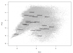
Figure 3: PCA dimension reduction solution for a 12-variable climate normal data set for the BC coast. The CWHwh1 and wh2 are incorrectly placed at the centre of the reduced climate space.
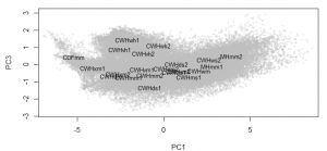
Figure 4: Third dimension of the PCA solution for the coastal data set, revealing that the CWHwh1 and wh2 are actually at one extreme of the full climate space.
The PCA solution for the coastal data set is shown in Figure 3 and Figure 4. The first three principal components represent 97% (58%, 33%, and 6%, respectively) of the variance in the data, which indicates that the data have an effective dimensionality of three despite being made up of 12 variables. PC1 and 2 provide a reasonable representation of the relationships between BEC variants, but incorrectly place the CWHwh1 and wh2 (Haida Gwaii) at the centre of the distribution. A third dimension (PC3) is required to correctly show that these variants are at one extreme of the distribution (Figure 4). The interactive 3D plot (Figure 5) shows that the normalized coastal data set has a dome-shaped distribution. This dome shape is a 2D manifold in 3 dimensions, plus noise. A successful non-linear solution would flatten this manifold into two dimensions and show the CWHwh1 and wh2 at the edge of the distribution. This criterion provides a means of evaluating how well LLE performs on real climate data.
Figure 5: 3D interactive plot of the LLE solution (use mouse to drag and zoom)
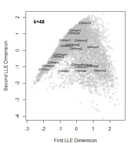
The LLE solutions for the coastal data set are shown above. LLE on small neighbourhoods (k=3, k=12) did not provide stable or meaningful solutions (Figure 6). Large neighbourhoods (k=48, k=200) produced functionally equivalent solutions. The k=48 solution (Figure 7) exhibits the desired behaviour of placing the CWHwh1 and wh2 at one extreme of the distribution while maintaining the CDFmm and the MHmm2 at opposite extremes. The
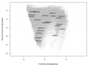
rank positions of the other BEC variants also make sense for the most part, although the relative proximity of the CWHds2 to the MHmm2 is problematic. Despite these apparent successes, the distribution of observations appears compressed towards the hypermaritime variants. Similar distortions appear to be common with LLE, even in showcased solutions on idealized data sets (e.g. Saul and Roweis 2003). This compression is extremely problematic for climate change visualization, because the magnitude of change will be exaggerated in some areas of the reduced climate space, and diminished in others. In comparison to an LDA solution (Figure 8), the LLE solution is not as satisfying.
Discussion
The goal of LLE and many other non-linear dimension reduction methods is to reduce manifold structures down to the intrinsic dimensionality of the manifold itself, i.e. to “unroll the jelly roll”. It is likely that climate data have a roughly manifold structure, because the observations are taken across a two-dimensional geographic surface and thus the distribution in climate space is likely to be constrained. However, the usage of LLE and other manifold learning algorithms for multivariate climate surfaces doesn’t appear to have been validated in the literature. Even if climate surfaces have a non-linear manifold structure (e.g. the dome shape evident in the three-dimensional PCA and LDA solutions for coastal BEC variants), that structure may have important climatic and ecological meaning. It means that some climate variables are important in some areas of climate space but not in others. As with the spiral experiment, linear methods will preserve non-linear relationships in the data space, and this may be a desirable result for visualization at regional and subregional scales.
LLE results are likely to be much more difficult to interpret in terms of the original input variables. LLE dimensions can be correlated with the raw variables of the full data space. However, these correlations could potentially have large variations across the distribution of data in the reduced data space. Also, it would be entirely possible for one LLE dimension to be correlated with two entirely uncorrelated climate variables. As a result, interpretations of the climatic meanings of the LLE dimensions would be unreliable, notwithstanding measures such as correlation mapping across the reduced climate space.
From a practical perspective, my project requires the ability to project new data into the reduced climate space. It is unclear whether it would be possible to map new data in an LLE-reduced data space. However, mapping of new data is feasible in other non-linear methods (Hsieh and Cannon 2008). Another essential practical consideration is that the computational requirements of LLE are prohibitive at anything larger than the regional scale. My computer could not run LLE on more than 10,000 observations, even using small neighbourhoods (k<12). This limitation makes LLE unfeasible for everyday use.
Despite these potential pitfalls, non-linear methods such as LLE have the potential to map the distances between observations regardless of the dimensions in which those distances occur. This is potentially a very useful feature for visualizing the magnitude of climate change, even if it obscures the climate variables in which those changes are occurring. Non-linear dimension reduction methods should be further evaluated, alongside mainstream linear methods.
Conclusion
The strength of non-linear approaches in theory is that they have the potential to map the distances between observations regardless of the dimensions in which those distances occur. In theory, this could produce multivariate data mappings at lower dimensionality than would be possible with linear methods. This is potentially very important for climate change visualization at provincial or continental scales, where there are likely to be many more than three important dimensions of climatic variation. The two analyses presented here confirm that LLE is able to extract a lower-dimensional manifold from higher-dimensional data, even on real, noisy climate data. However, LLE appeared to create non-linear distortions in the reduced data space, which is a severe drawback for climate change visualization. In addition, interpretation of LLE dimensions is confounded because they can be made up of uncorrelated variables. Finally, LLE is extremely computationally intensive. Non-linear dimension reduction approaches deserve further investigation due to their theoretical advantages, but this case study of LLE suggests that the search for an appropriate method may be very time-consuming. Linear methods such as LDA and PCA appear to be adequate at the regional scale. For the moment, I will focus on my immediate research objectives, and return to non-linear methods at a later date.
References
Hsieh, W. W., and A. J. Cannon. 2008. Towards Robust Nonlinear Multivariate Analysis by Neural Network Methods. Lecture Notes in Earth Sciences 112:97–124.
Ridder, D. De, O. Kouropteva, O. Okun, M. Pietikainen, and R. P. W. Duin. 2003. Supervised locally linear embedding. Pages 333–341, Artificial Neural Networks and Neural Information Processing — ICANN/ICONIP 2003.
Roweis, S. T., and L. K. Saul. 2000. Nonlinear dimensionality reduction by locally linear embedding. Science 290:2323–6.
Saul, L. K., and S. T. Roweis. 2003. Think Globally , Fit Locally : Unsupervised Learning of Low Dimensional Manifolds 4:119–155.

