Visualization of historical and projected future climate change at Blind Channel, BC.
Summary
This blog post is a test run of a linear discriminant analysis (LDA) method for climate change visualization. The objective of this analysis is to create a low-dimensional (2D or 3D) climate space that reasonably represents the geographic variation of climate on the BC coast, and use that climate space to contextualize historical climatic variability and projected climate changes at selected locations. The analysis produced following outcomes:
- LDA appears to have produced a meaningful reduced climate space that reasonably represents the relationships between BEC variants. The regional scale appears to be more appropriate than the local (transect) or provincial scale;
- The backdrop of regional climatic variation provided a useful context for historical interannual climate variability and projected climate changes. However, projections into regionally novel climate space were difficult to evaluate due to absence of potential climatic analogs from outside the region;
- There appear to be dramatic sub-regional differences in the scale and novelty of projected climate change. Climate change on the north coast appears to be relatively moderate, and stays within the existing range of regional variation. In contrast, climate change on the south coast appears to be of much greater magnitude and entirely into regionally novel conditions.
The key next steps are to develop and test-run other alternative dimension-reduction methods such as multidimensional scaling, and to develop methods to visualize distant climatic analogs and truly novel climate space.
Introduction
In a previous blog post I discussed the results of a discriminant analysis of BEC variants along an elevational transect in central interior of BC. My conclusion was that only the first discriminant axis was meaningful. The other axes represented non-linearities in the relationships between the climatic variables, and did not have an intuitive climatic interpretation. As a result, discriminant analysis, though useful for classification, is likely of dubious value as a method for creating low-dimensional climate visualizations in a simple climatic gradient. Nevertheless, I was curious how discriminant analysis performs on a larger and more complex climatic landscape. It is possible that meaningful variation in the second and third dimensions will relegate problematic non-linearities to lesser dimensions.
The purpose of this blog post is to test run an LDA-driven climate change visualization at a regional scale. I do a discriminant analysis on the 1961-1990 climate normals over a 1600-metre grid of coastal British Columbia. The results are evaluated in 2D and 3D climate space. Then I plot historical interannual variability and projected climate change for individual locations to get a glimpse of what climate change visualizations might look like in the reduced climate space.
Biogeoclimatic Climate Classification for the Coast
The coastal region provides a good case study because it has a relatively simple climatic geography, compared to the interior of BC. The climatic variation of the coast can be understood in a simple sense in terms of four climatic gradients:
- dry in the south vs. wet in the north, due to the influence of the Aleutian low;
- wet belts and rainshadows associated with the mountains of Vancouver island, the Olympic Peninsula, Haida Gwaii, and the Coast Range;
- hypermaritime (low seasonality of temperature) on the outer coast vs. submaritime (hot summers, cold winters) inland, due to the moderating influence of the Pacific Ocean; and
- Decreasing annual temperatures with elevation.
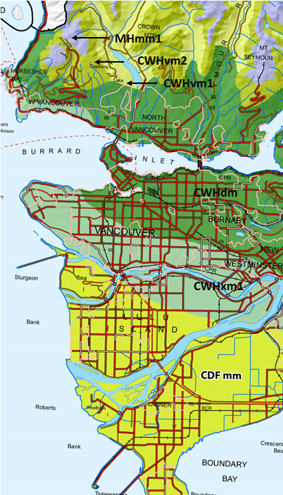
Figure 1: An example of the BEC climate classification: BEC variants of Vancouver BC.
The Biogeoclimatic Ecosystem Classification (BEC) includes a detailed classification of the climates of the coast. The naming conventions of the BEC climate classification of are simple to understand and worth knowing. The vast majority of the coast is classified as the Coastal Western Hemlock Biogeoclimatic Zone. The exceptions are the Coastal Douglas-Fir (CDF) zone in the mediterranean climate of the Georgia Basin, and the Mountain Hemlock (MH) zone in subalpine elevations. Subzones are named with a two-letter code corresponding to their relative precipitation (x=very dry, d=dry, m=moist, w=wet, v=very wet) and continentality (h=hypermaritime, m=maritime, s=submaritime). Each subzone generally has at least two variants. In the CWH, variants are either elevational (1=submontane, 2=montane; CWHmm/vm/wh/ws) or latitudinal (1=southern, 2=central; CWHds/ms/vh). In the MH zone, variants are windward (1) vs. leeward (2). Figure 1 shows a small portion of the BEC variant mapping of the coast to provide a sense of the scale of the BEC climate classification.
Methods
Observations are locations on a 1600-m grid clipped to the geographic range of the CWH, CDF, and MH zones (MHmm1/2 only). I used the following annual climate normals output from ClimateWNA: MAT, MWMT, MCMT, TD, MAP, MSP, AHM, SHM, DD_0, DD5, FFP, PAS, Eref, and CMD. I log-transformed precipitation and heat-moisture variables (MAP, MSP, AHM, SHM, PAS) to normalize their distributions. LDA was done on these data using the “lda” call in the MASS package of R.
Results
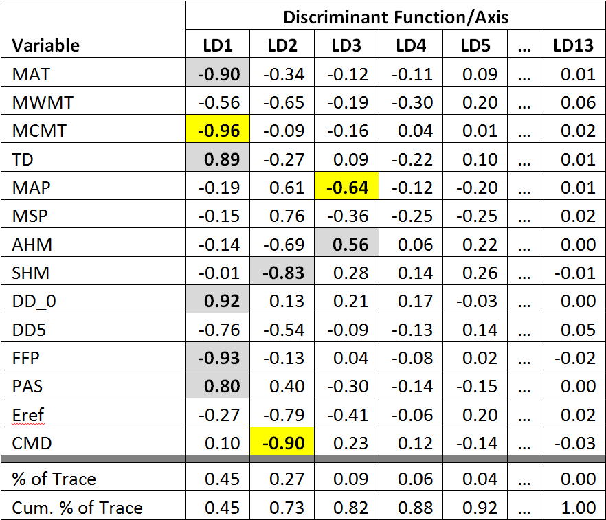
Table 1: Correlations between climate variables and the first 5 of 13 linear discriminant functions. Primary correlations are highlighted grey, and the leading correlation is highlighted yellow. “% of trace” is an unrelated index of the percent of between-class variation explained by each discriminant function.
The structure of the LDA is strikingly different from that of the Quesnel-Barkerville transect. The first three discriminant functions (LD1-3) explain a moderate 82% of the between group variance of the coastal BEC variants (bottom of Table 1), which was the same amount explained by LD1 alone in the Quesnel-Barkerville transect. This is no doubt because the coastal region contains many climatic gradients, rather than just one. The correlations between the major discriminant axes (Table 1) are also more easily interpretable than in the transect analysis. LD1 appears to be an index of cold winters, and LD2 appears to be an index of growing season moisture availability (i.e. a negative drought index). LD3 appears to be a negative index of precipitation, especially of winter precipitation.
2D visualization of the coastal climate space
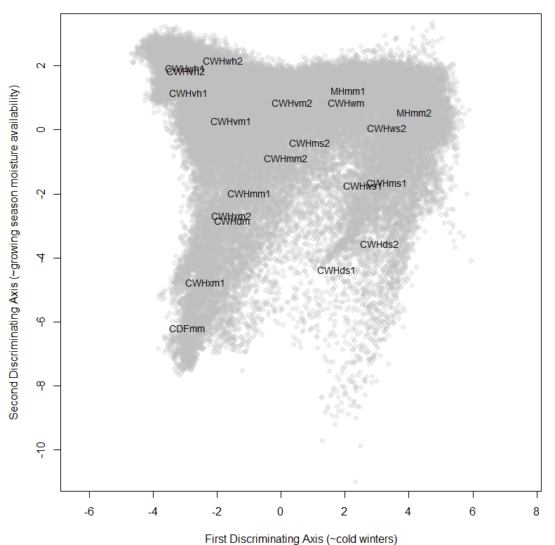
Figure 2: Simplified plot of the coastal grid in the first two discriminant axes, with BEC variants labelled at their climatic centroids.
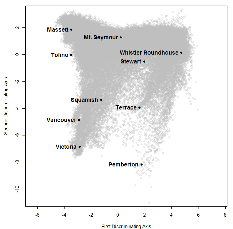
Figure 3: ClimateBC normals for some reference locations
The relative positions of the BEC variants in the first two dimensions make sense in the context of these climatic indices (Figure 2). The progression from the bottom left to top right (CDFmm to MHmm1) is essentially the sequence of BEC variants moving outwards from the Georgia basin and upwards into the mountains of Vancouver Island and the coast range. The progression from the bottom right to the top left (CWHds1 to wh1) is the sequence of BEC variants from the coast-interior transition zone to the outer coast. The gap between the maritime and submaritime BEC variants in the first dimension is likely due to the presence of the coast mountains; i.e. the narrow glacial valleys connecting these two groups do not contribute enough grid points to fill the transition. The only pairing of BEC variants that doesn’t make sense in the first two dimensions is the CWHwm (sea level) and MHmm1 (subalpine). Overall, this appears to be a valid low-dimensional representation of the coastal climate space.
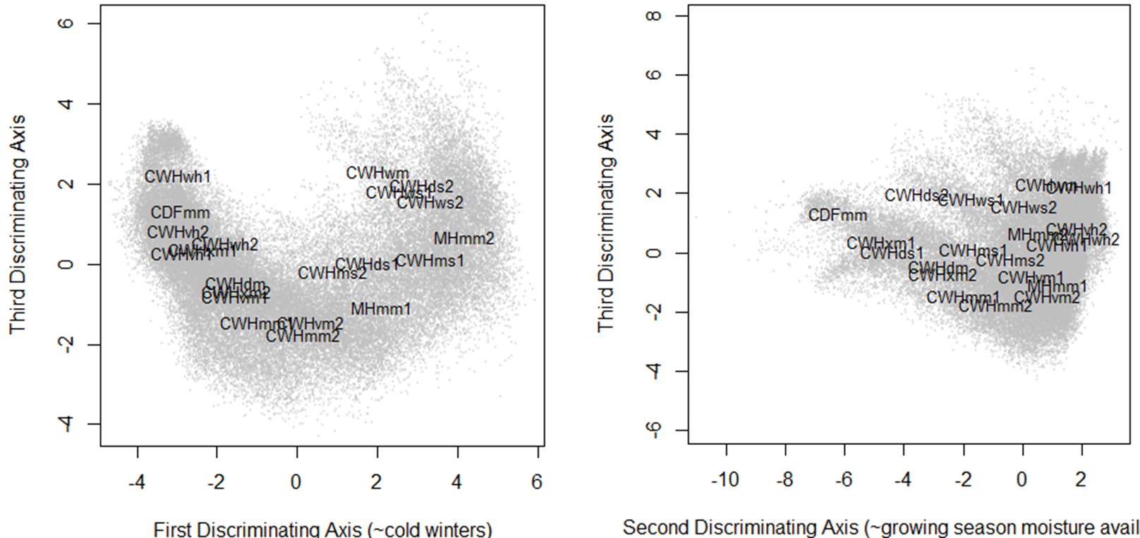
Figure 4: Grid points in the third discriminating axis plotted against the first and second axes.
The third dimension of the coastal discriminant climate space is shown two-dimensionally in Figure 4, and below as an interactive three-dimensional visualization. There is a pronounced three-pointed arch shape in the third dimension. However, it is not clear whether this is a cryptic artifact of non-linearities in the data, or a meaningful climatic phenomenon. The correlation structure of the LDA (Table 1) suggests that the third axis is an index of winter dryness. The plot of the second and third dimensions (Figure 4, right) clearly distinguishes the rainshadows of the Olympic Peninsula/Vancouver Island (CDFmm), the Coast Range (CWHds2/ws1), and Haida Gwaii (CWHwh1). Interestingly, the CWHvh1 and vh2 also have intermediate values in the third dimension. This result makes sense, despite the common misconception that the hypermaritime subzones experience the highest rainfall on the coast; large areas of the CWHvh1 and vh2 are outer coastal lowlands that experience more summer fog than adjacent maritime subzones (e.g. CWHvm1) but less frontal precipitation due to the lack of orographic uplift. The CWHwm and MHmm1, which were poorly discriminated in the first two dimensions, are well discriminated in the third dimension. Despite the consistency of these observations with patterns of winter precipitation, the arch-shaped relationship between the first and third dimensions is questionable. It would take further investigation to determine whether this relationship is cryptic or meaningful. For this reason, I use only the first two dimensions for the remainder of the analysis.
Interactive 3D visualization (drag and zoom to explore the climate space)
Distribution and overlap of BEC variants within the climate space
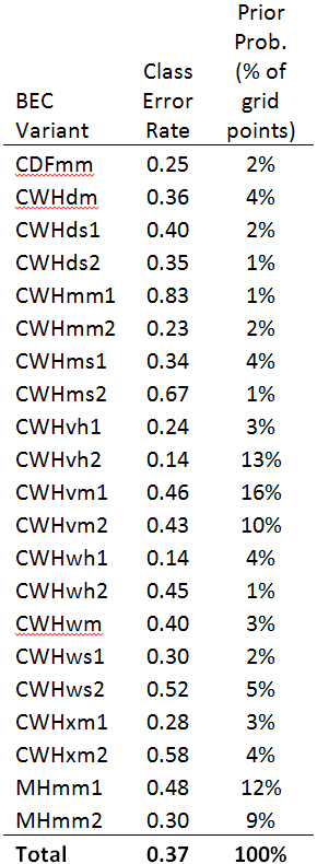
Table 2: Classification error rates of the discriminant analysis, indicating the number of grid cells that fell within another BEC variant’s domain in full-dimensional climate space. Prior probabilities are simply the proportion of the total number of 1600-m grid cells in each BEC variant.
Figure 6 shows the distribution of grid point normals for three arbitrarily selected BEC variants. The grid points of each BEC variant are disperse widely through the first two dimensions, and overlap with numberous BEC variant centroids. Superficially, this suggests low accuracy of the BEC variant mapping and/or of the ClimateWNA/PRISM data. However, the classification error of the discriminant analysis is 37% (Table 2). This indicates that almost 63% of the area of the BEC variants fall into their own exclusive region of the full-dimensional climate space. The remaining 37% classification error is a combination of errors in the BEC variant mapping, ClimateWNA/PRISM surfaces, and variable selection, in unknown proportions. These results indicate that ClimateWNA data can reasonably differentiate BEC variants in full-dimensional climate space, but that differentiation in low dimensional climate space is poor. The climatic centroid of BEC variants is likely much more meaningful in reduced dimensions than the boundaries between BEC variants.
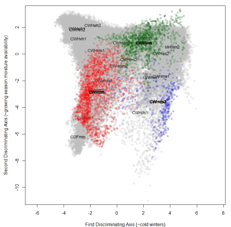
Figure 5: Spatial variability of ClimateBC output for three BEC variants.
Visualizing historical and projected climate change in the 2D discriminant climate space
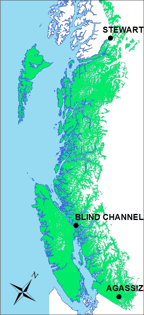
Figure 6: locations of the weather stations used for the climate change visualizations. The distribution of the Coastal BEC zones is shown in green.
The locations of three long-term weather stations were selected as case studies for climate change visualization (Figure 6). These sites roughly represent the northern, central, and southern regions of the BC coast, though Blind Channel is in an area that is climatically transitional between the southern and central regions. Although these are weather station locations, it is important to note that all date presented here is from ClimateWNA.
The graph for Stewart (Figure 7) can be used to introduce the elements of the climate change visualizations. The case study location is labeled at the position of the 1961-1990 normals in climate space. The climatic conditions of individual years in the period 1951-2010 at the case study location are shown as empty blue circles. A 30-year moving average of these years, shown as a blue line, shows the drift in climate normals starting with the 1951-1980 normals, and ending with the 1981-2010 normals. Future climate normals projected by two GCMs are shown as red dots and labelled by median year. The red dotted line is a spline interpolation with no climatic meaning except to visually connect the projected normals. Collectively, the intent of all these graphic elements is to contextualize GCM projections in terms of historical climatic variability and regional climatic variation.
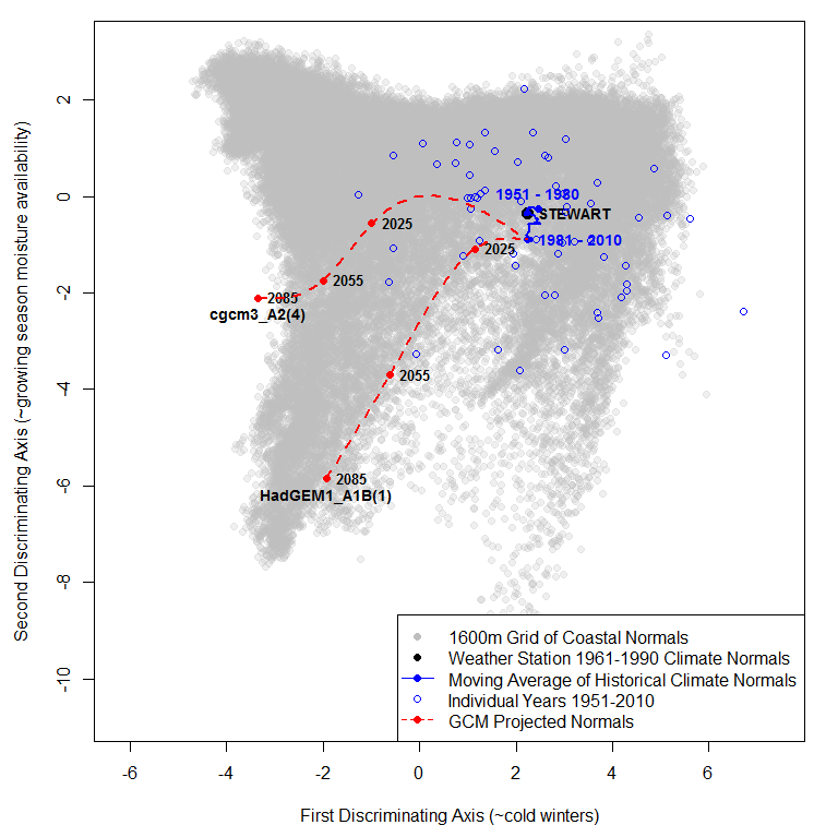
Figure 7: Historical climatic variability and GCM-projected climate change at Stewart, BC.
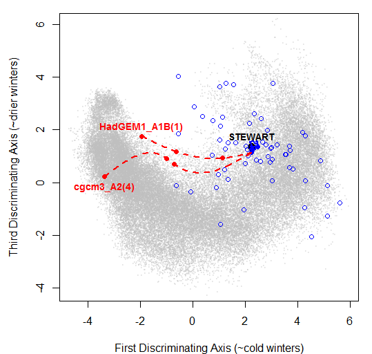
Figure 8: GCM projections for Stewart BC in the third discriminant dimension
Historical interannual climatic variability at Stewart is substantial, though the range of variability generally falls within the 2D climate envelope of the coast. Despite this interannual variability, climate change has been limited over the past 60 years at Stewart, as suggested by the blue moving average of climatic normals. Nevertheless, there is a trend towards droughtier conditions. Neither of the GCM runs project a continuation of drying trend in the 2011-2040 normal period (labelled “2025”). Instead, they both project a moderate to rapid shift towards warmer winters initially, then a shift towards warmer winters and droughtier growing seasons. Within the 2D climate space, there are historical climatic analogs for the end point of both projections: conditions in the 2071-2100 normal period (labeled “2085”) are similar to the 1961-1990 climate normals for Agassiz the HadGEM1_A1B(1) run and for Port Renfrew in the cgcm3_A2(4) run. These analogs also apply in the third dimension (Figure 8).
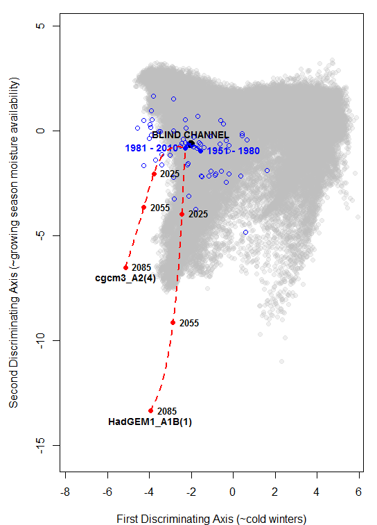
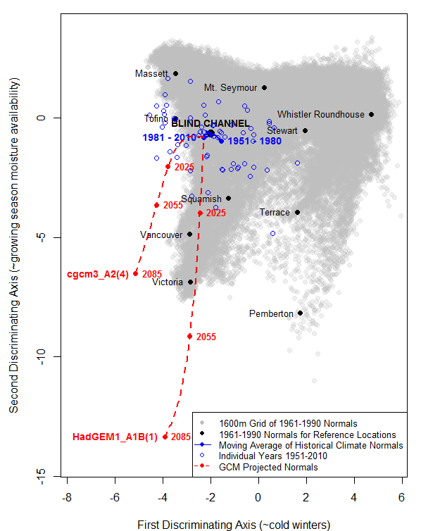
Figure 9: Historical climatic variability and GCM-projected climate change at Blind Channel, BC.
The other two case studies are more than 5 degrees of latitude south of Stewart, and in the neighbouring GCM grid cell. Projected climate changes in these two case studies are more dramatic, especially at Agassiz. The endpoint of both GCM runs is entirely novel to the coast, and well beyond the range of interannual variability over the past 60 years. It is worth noting here that a climate envelope classification based on discriminant analysis would likely classify these novel endpoints as CDFmm due to the lack of available analogs.
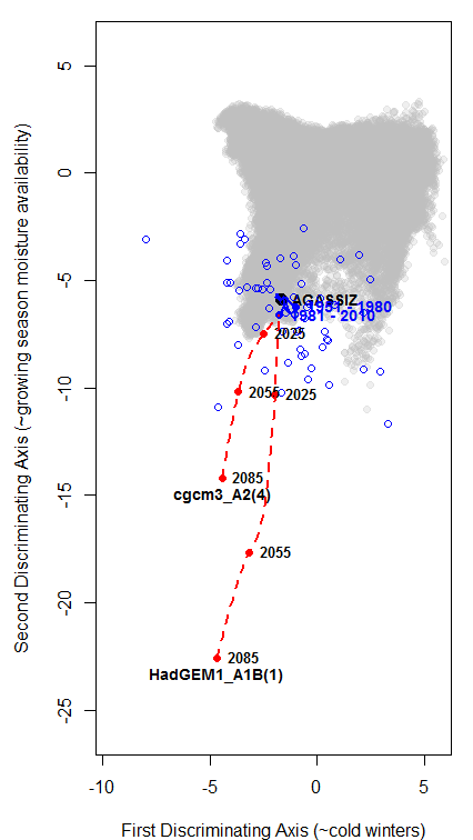
Figure 10: Historical climatic variability and GCM-projected climate change at Agassiz, BC.
The most striking pattern of the three case studies is that the apparent scale of climate change is dramatically greater in the south coast. Whether or not this reflects the relative scales of climate change in the GCM runs is yet to be investigated. The most likely reason for this effect is that the second discriminating axis exaggerates changes towards progressively drier conditions. This is entirely possible because CMD was not log-transformed even though it is partially derived from precipitation. To check this hypothesis, I reran the analysis without CMD and Eref. Surprisingly, the results were very similar. Further investigation is required to determine whether the second axis contains distortions that exaggerate climate change in drier areas of the climate space.
Overall evaluation of the method
The purpose of this analysis was to create a low-dimensional (2D or 3D) climate space that reasonably represents the geographic variation of climate on the BC coast, and use that climate space to historical climatic variability and project climate changes. Was the method successful? Here are my thoughts:
- Discriminant analysis of the 1961-1990 normals of the 1600m grid locations produce a 2D climate space that reasonably represents the relationships between BEC variants, with some exceptions. These exceptions were resolved in the 3D climate space. It is likely that this reduced climate space could be improved through careful variable selection and transformation. Notably, CMD is calculated from climate normals in ClimateWNA, which skews its distribution towards zero. For this reason, CMD (and its precursor Eref) should be either dropped from the analysis or recalculated from monthly observations.
- The dimensions of the reduced climate space for the coast are climatically meaningful, and are relatively free of the cryptic artefacts that drove the second and third dimensions of the Quesnel-Barkerville transect. This indicates that there is a “goldilocks”-type sweet spot for the scale of study areas for reduced climate spaces. Transects are too small, because they only represent a single axis of climatic variation. The province is too big, because it contains many important axes of variation that cannot be meaningfully represented in 2D or 3D. The regional scale appears to be “just right”. Of course, it is unclear whether the “novel conditions” portrayed in the case studies are truly novel or just regionally novel. This is the tradeoff between local vs. global classification that I discussed in the previous blog post. Nevertheless, it may be possible to resolve this tradeoff with the right method.
- This background of regional variation provides a useful context for interannual variability and climate change. However, the (possibly fatal) flaw of this approach is that it constrains the representation of climate variability and change to the primary dimensions of existing geographic variation (winter temperature and summer drought in this case). Variation in other dimensions is invisible, even though it may be highly biologically relevant. This is a potential problem in situations like the visualization for Stewart, where there appeared to be climatic analogs for the projections in 2D and 3D space. It is much less of a problem where novel conditions are projected in 2D, as in Blind Channel and Agassiz, since it is highly unlikely that analogs would exist in full-dimensional climate space that don’t exist in the reduced space.
- Projections of climate change into novel areas of the climate space are visually dramatic. However, the discriminant axes may conceal non-linearities that distort the representations of these changes. Any axes created through discriminant analysis require extensive validation.
- This analysis was primarily an exercise in visualization. In order for the method to be successful, however, it must also facilitate quantitative analyses of climatic variability, differentiation, and novelty. I’m not yet convinced that discriminant analysis provides reliable axes (metrics) for quantitative purposes.
Next steps
- Develop and test-run some other methods for achieving the same objective. The most obvious alternate approach is multidimensional scaling. Another alternate approach is to use LDA or some other method to assist with supervised variable selection, and use raw climatic variables as visualization axes. For example, it appears from this analysis that MCMT, SHM, and MAP may be viable first, second, and third axes for a more intuitive reduced climate space for the coast region. Ultimately, the method must be compatible with a quantitative analysis of climatic variability, differentiation, and novelty (a la Williams et al. 2007).
- Develop methods to resolve the compromise between local and global classifications. An example of a potential approach is a two-step graphical approach. The first graph would plot grid points for the entire western North America in the discriminant axes of the coastal climate space and portray GCM projections for a focal (BC coastal) location against this background. The axes of the second graph could be the discriminant axes for the climatic analog (Oregon? California?) for the projected conditions of the focal location. This approach would provide a graphical validation of the inferred analog. Localized LDA (described in the previous blog post) may be a viable method for this approach.
- Evaluate the pros and cons of including interannual climatic variability and the GCM projections into the discriminant (or alternate) analysis. The advantage would be that the reduced climate space could portray key axes of temporal variability that don’t exist in the geographic climatic variation. The disadvantage is that it may be difficult to simultaneously represent spatial and temporal variability in a reduced climate space at the regional scale. This approach may only be viable for transects.
References
Williams, J. W., S. T. Jackson, and J. E. Kutzbach. 2007. Projected distributions of novel and disappearing climates by 2100 AD. Proceedings of the National Academy of Sciences of the United States of America 104:5738–42.