01/28/18

The Homebrew series: Novel climates in BC, by Colin Mahony et al.

The year got off to a flying start in the Aitken lab, with a Forest Ecology and Management publication from our own Colin Mahony and his collaborators. Basically, if everyone else’s year started on a rocket, it’d better be running on clean energy. Following on his recent Global Change Biology publication, Colin shows us that human induced climate change is no joke to our beloved BC forests, and the future might be more grim than previously anticipated by forest managers. Colin shows that novel climates, climates that are currently not experienced anywhere in BC, might arise in BC by mid-century, and that these unprecedented conditions may fall under the radar with the current use of the BEC projection model.

At the moment, the best way to decide what forest tree species to plant where is to project ourselves forward about 50 years (about the time it takes for forestry trees to become fully mature) and determine what climate will be occurring then in the area of interest. Tree species and provenances can then be selected from BC areas with the closest contemporary climate. This is all done through the BEC system, which groups BC climatic conditions in an ecologically meaningful set of units.

The crucial question is: what if there is no place in BC that matches the predicted future climate of an area? Should we expand our range to all of North America? Well, Colin et al. actually show that some mid-century novel climates of BC have no equivalent in other parts of North America either…

These results highlight the limitations of the BEC projection model: 2 of the measures of the method, analog similarity and ensemble agreement, are actually diagnostic of novel climates at high values. In other words, projections of future BEC climates can be erroneous in novel climates, in particular by creating an appearance of reduced climate disruption and uncertainty. In providing a map of where novel climates are likely, this research points to regions where BEC projections are reliable from areas where other analytical approaches are required.

Here’s what lab members reading the paper had to say about it:

What’s our takeaway from this paper?

We don’t know what we think we know about future climate/ecology predictions in lowlands, coastal regions, and NE BC, because the climates there are unlike all others in North America. Forest management practices should rely on a species-specific basis, and be adapted with new management approaches—not found in other BEC zones’ practices.

“The best match is not necessarily a good match.” Depending on the analog pool, amount of climate change, and particular decision framework you use, you may find that the best climate analog is nothing like the actual climate. If I’m picking my pants from the kids section, the biggest ones are the best fit, but I can still only get one leg in them!

What’s the coolest thing about this paper?

Standardizing changes in climate by interannual variablility is a really cool way of expressing their ecological relevance, and if you want to know more about this smart method, check out Mahony et al. 2017. Also, despite the uncertainties in predicting the future of ecosystems under climate change, this study presents a fine-scale adjustment on what was known and on what was expected for British Columbian forests under climate change. The provided information will be key to reducing the risks of resource losses in the province.

Figures 2 and 3 are such awesome figures. They clearly and concisely explain a concept that can be difficult to get your head around.

What question are we left with after reading this paper?

What would the scenario of novel climates be on a global scale using the same approach?

What management methods should we use in areas where novel climates are predicted to occur?

Is Colin’s middle name Reginald? Rudolphus? Royce? An enduring mystery…

I didn’t really understand the pros and cons of the linear novelty detection method vs random forests on first read and was pretty confused trying to interpret the random forests figures. I’d love to see a talk breaking down the random forests method and results in isolation. Or maybe I should just read the supplementary material?

Reading climate novelty papers like this makes me want a tool that lets me plug in coordinates, a year and an emissions scenario and get a map of climate analogs and their associated ecosystems.

12/1/17

Are you playing Secret Santa? a R function

We’re playing Secret Santa in my family: you are giving a present to only one other person, and their identity is only known to you. You need to give them a handmade present or a present bought in a second-hand store. Well that last part is our own variation of the concept.

You might be playing Secret Santa in your lab.

Here is a little R function to sort the draw without anyone seeing the outcome, and without the need to involve an external participant. The only inputs are:

-a vector of names of participants; for example c(“Patrick”,”Nicole”,”Maria”,”Pablo”)

-the folder where you want the output files; for example “C:/Users/Maria/SecretSanta”

After you’ve run the function, send to each person the output file named after them.

The function:

secretsanta=function(names,directory){
chosen=names
for (i in 1:length(names)){
 if (names[i]%in% chosen){
 choice=sample(chosen[-which(chosen==names[i])],1)
 }else{
 choice=sample(chosen,1)
 }
 chosen=chosen[-which(chosen==choice)]
 write.table(paste(directory,"/",names[i],", you will give a present to ",choice,sep=""),
 file=paste(names[i],".txt",sep=""),quote=F,row.names=F,col.names=F)
 }
 return("Done! the files are in the provided directory. Merry Christmas.")
}


Load the function into R by entering the code above, and then run the function with your input:

secretsanta(names=c("Patrick","Nicole","Maria","Pablo"), directory="C:/Users/Maria/SecretSanta")


Merry Christmas!


12/4/15

Scouring coastal Alaskan forests : a journey through the past (Part 2)

Two wonderful weeks of hard work on the Kodiak Archipelago resulted in a truck loaded with 350 silica-dried needle samples and about as many tree cores from Sitka spruce forests. Happy and satisfied with the amount and spatial distribution of these tree samples, I embark on the ferry full of confidence about the second part of the trip: Sampling on the Kenai Peninsula.

Kodiak Island from the ferry

Bye-bye Kodiak!

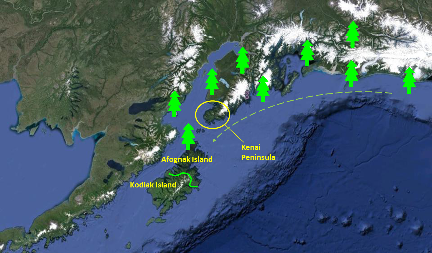
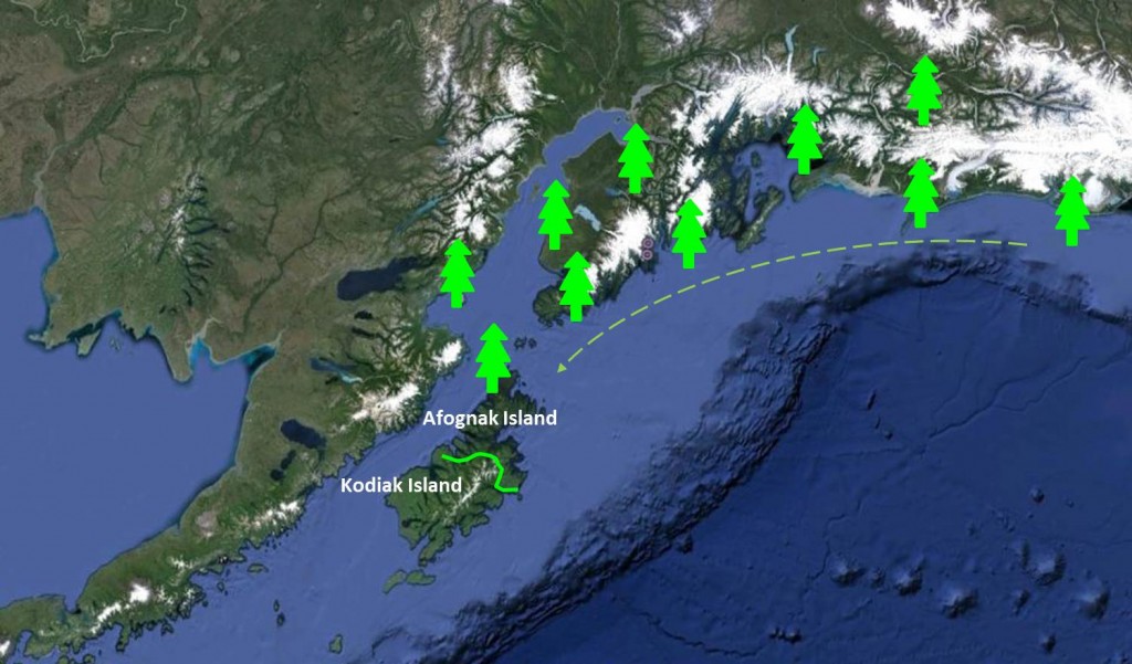
Back on the continent, my main objective is to find old-growth forests of Sitka spruce and apply the same sampling design. By doing so, I will be able to compare the genetic make-up of a long-established forest to the young forests of the Kodiak Archipelago. I chose the Kenai Peninsula because it is the most likely origin of the trees that established on Afognak and Kodiak Island.

map_expansion_2

Just to remind you the general direction of Sitka spruce expansion.

This second chapter to the Alaska journey will provide the essential baseline data for my project and will help answering the following questions:


To what extent is population expansion linked to a drop in genetic diversity?

Are trees at the front of expansion experiencing higher levels of inbreeding than trees in core populations? Are they subject to lower levels of selective pressure?

Do deleterious / advantageous mutations spread more easily during population expansion?

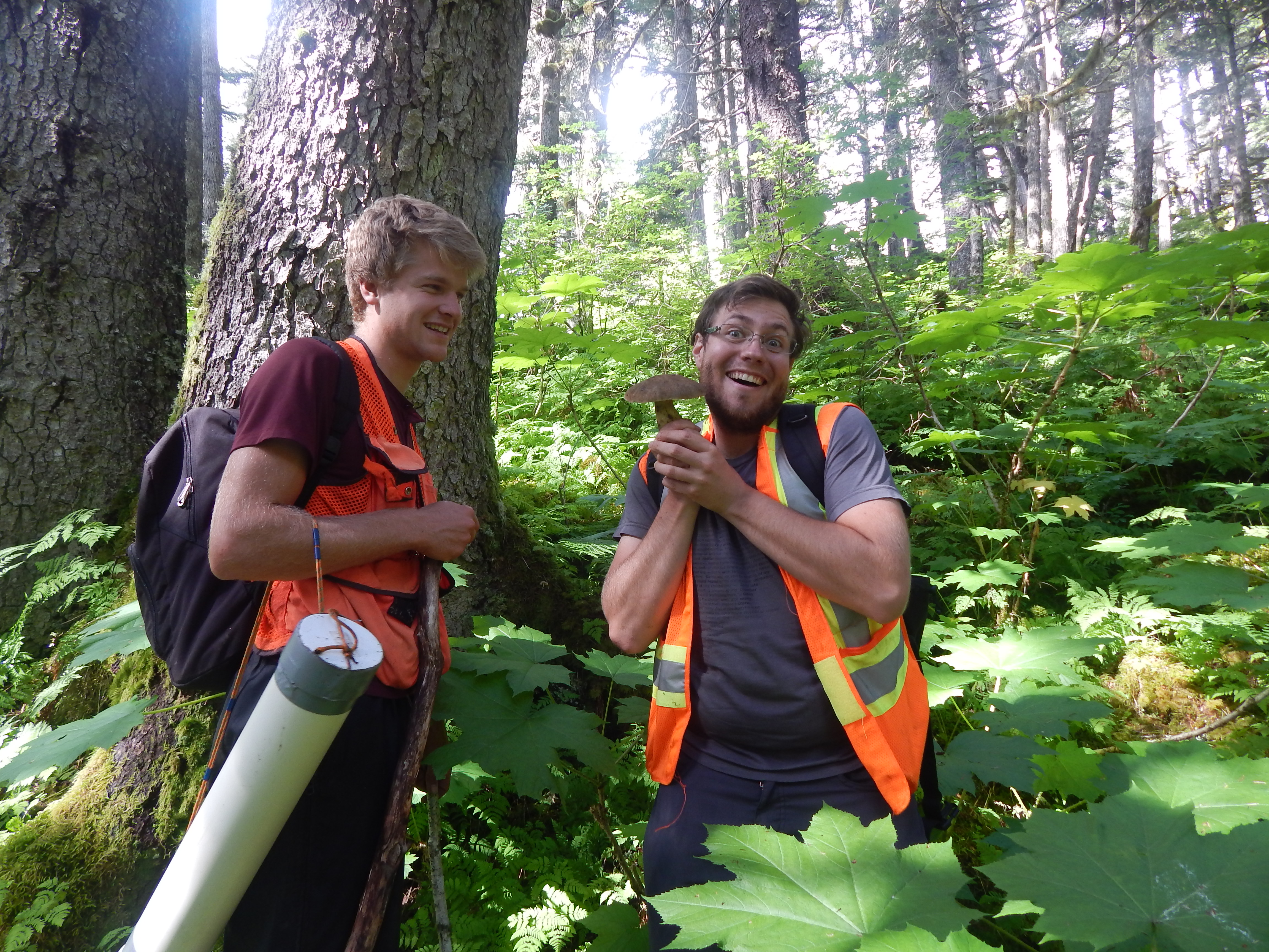
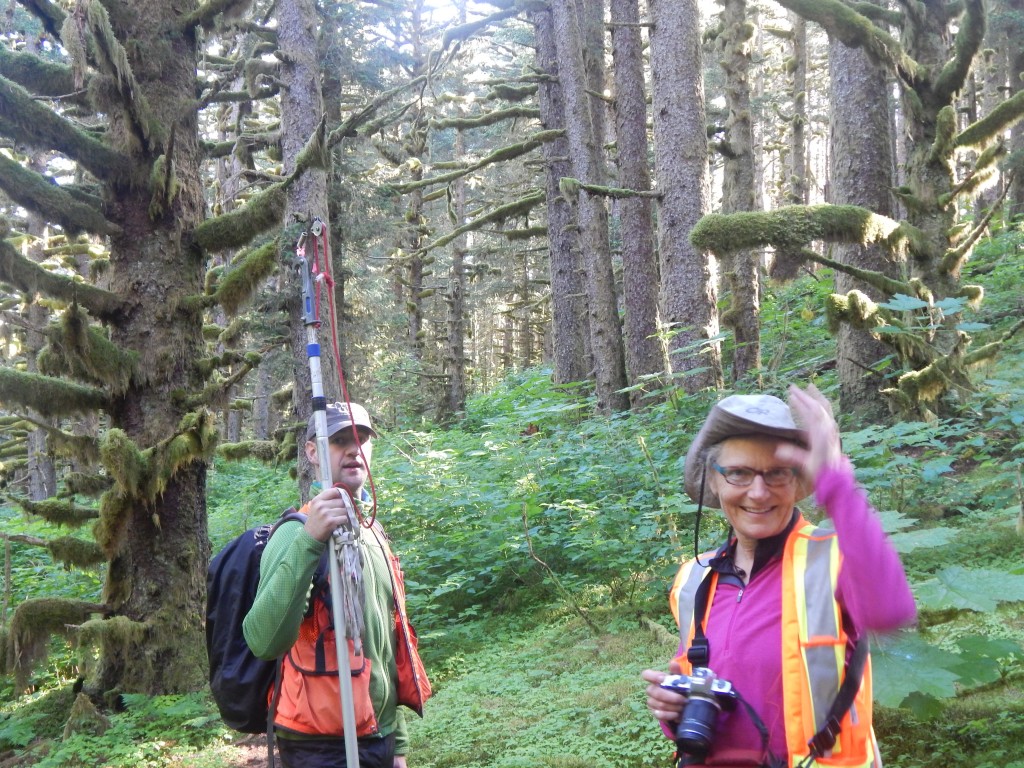
Team number 2 is waiting for me in Anchorage: Jon and Vincent, fresh out of the plane. Two highly motivated Aitken Lab members. Two masters of tree-spotting, mushroom-picking, blueberry-gathering, and wild-cooking. Already on the first day I am tempted to re-name them Witty and Cheeky. But they ended up being “Yonathaaan” (with the strongest German accent you can adopt) and “Young Padawan”.

Jon and Vincent.

The crème de la crème of mushroom pickers.

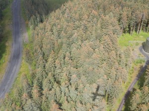
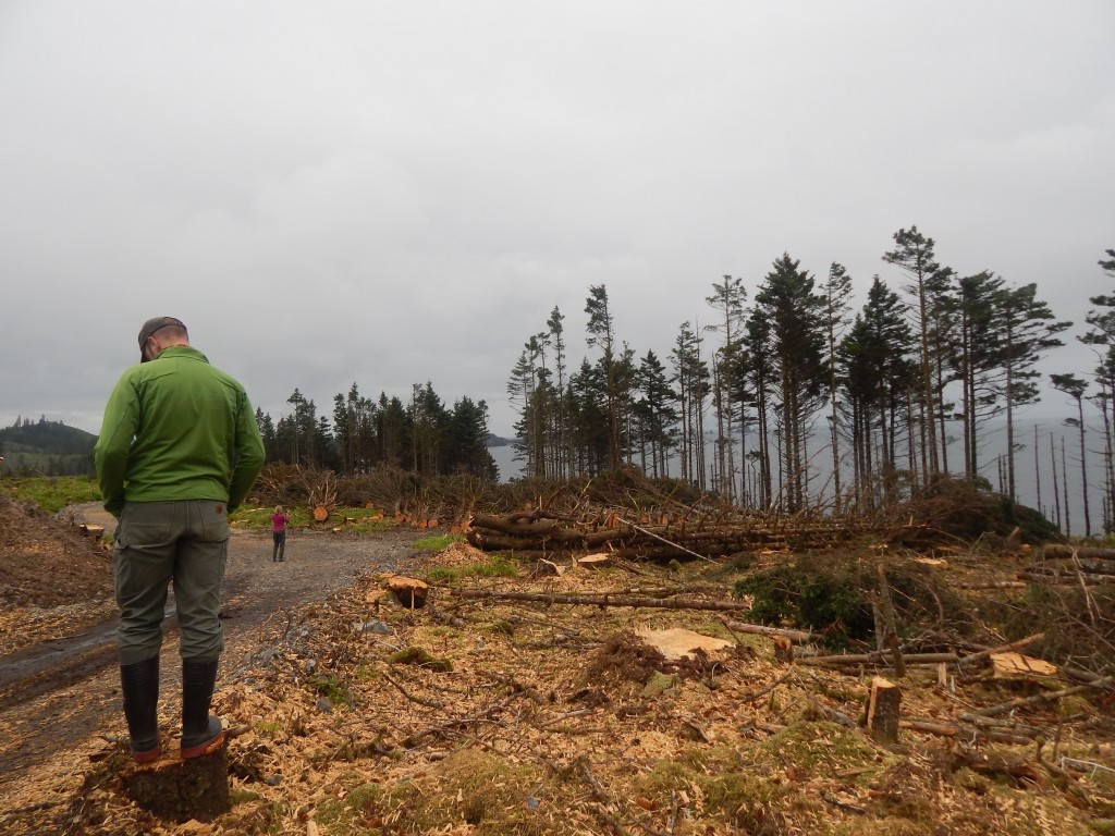
While the difficulty on Kodiak was to get to big trees before the loggers, the difficulty on the Kenai was to get to big trees before the bark beetle. A devastating outbreak in the 1990s left very little of the pristine, old-growth spruce forest I was looking for. A lot of remaining old-growth lies in a thin strip of wet lowland crunched between the sea and the gigantic Harding Icefield, an impossible target for us and Bean, who likes roads more than glaciers and waves.

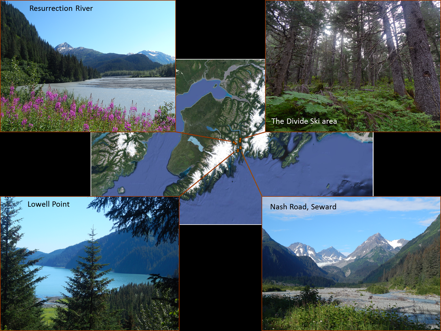
But thanks to the help of Ed Berg, bark beetle expert, John Morton, wildlife biologist, and our flawless determination, we finally manage to find beautiful, road-accessible stands of pure Sitka or mixed Sitka spruce-western hemlock forests around the Seward Inlet.

Kenai sampling areas

Sampling locations around Seward

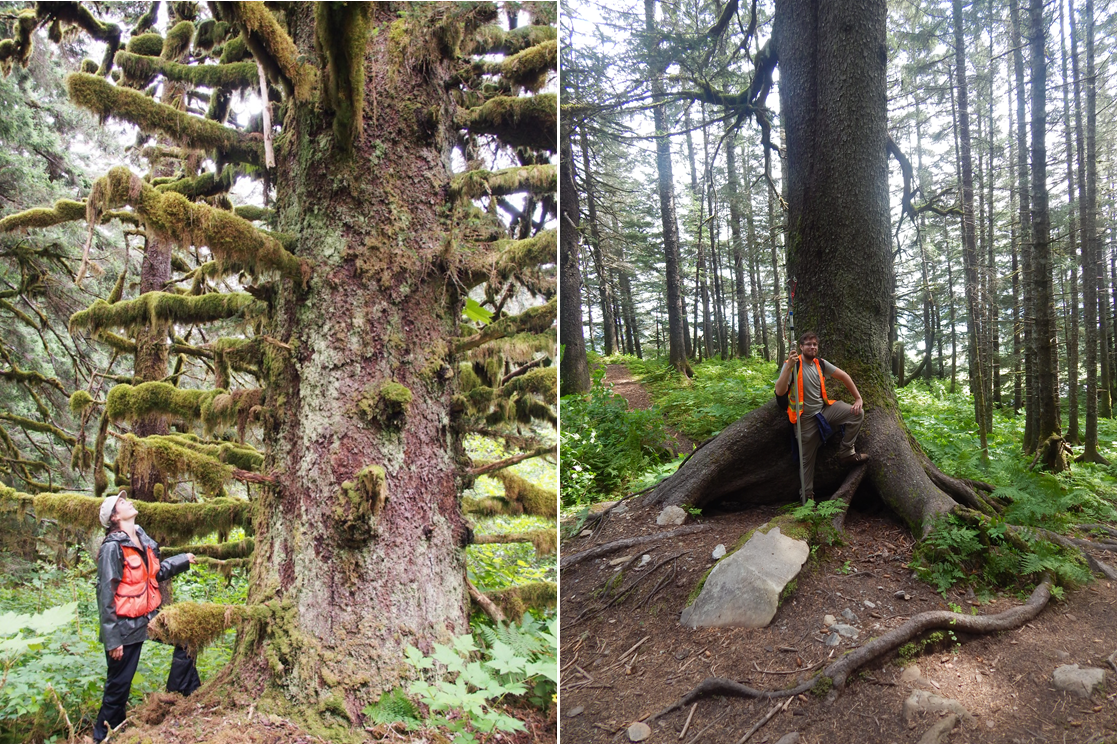
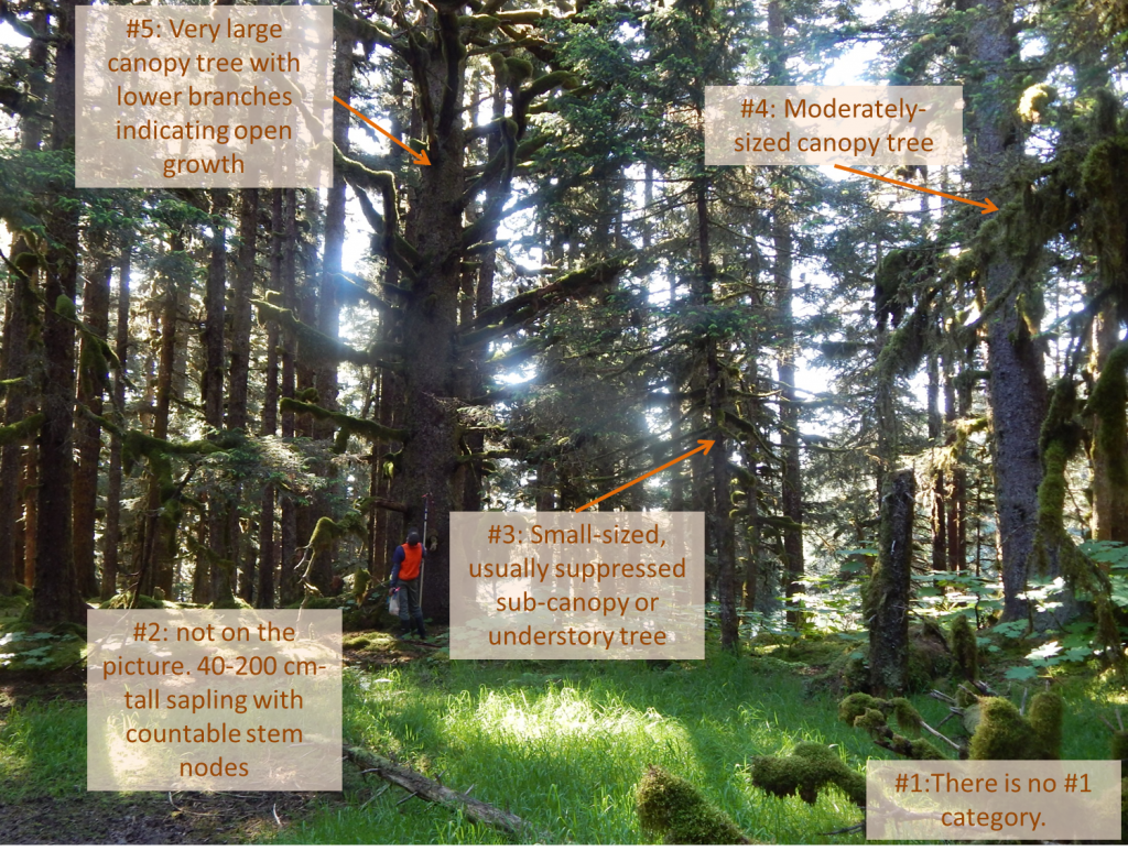
After stalling a few times due to excessive scenic landscapes, we’re back in the coring-trunks-and-snipping-twigs business! We keep the same sampling scheme as on the Kodiak Archipelago: collecting equal numbers of tree needle and tree cores among 4 levels of forest structure (see previous post for details) in several locations, and keeping a distance of at least 50 m between sampled trees. The most striking difference in forest structure with Kodiak Island is that there is no “proper” tree of level 5. For sure there are very large trees (winning DBH: 138cm!), but none of them shows signs of open-growth (large lower branches). To me, this confirms that the canopy on the Kenai is way older than the oldest trees, unlike the canopy of Kodiak Island.

take_five

On the left, a Kodiak #5. On the right, a Kenai #5. Note: the scale on both pictures is represented by a normal-sized human being.

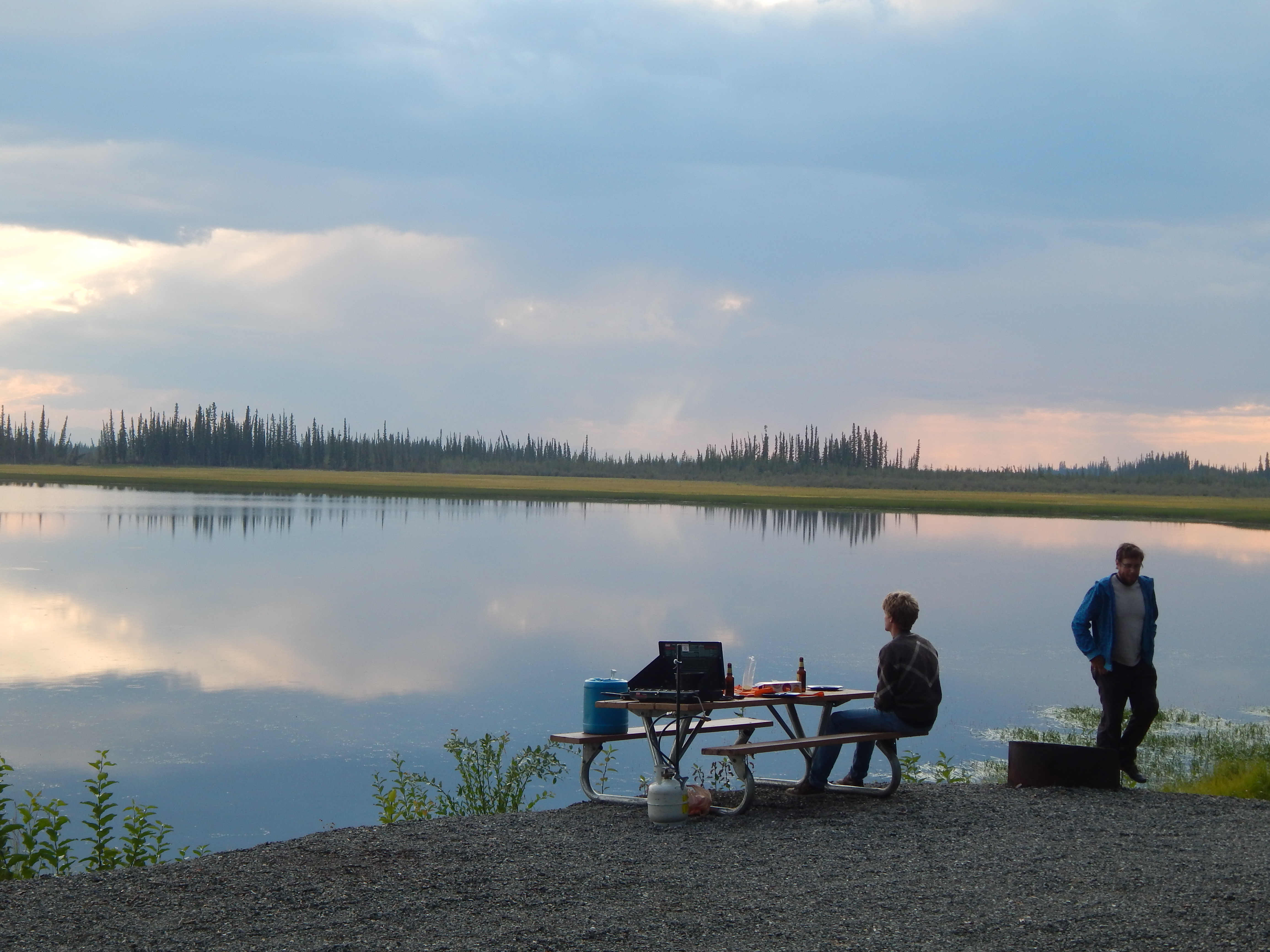
Although finding stands with no sign of recent disturbances was a real challenge on this part of the field trip, we managed to find four suitable sampling areas around the Seward inlet and added 197 trees to the collection. Early August, more than six weeks after having left from Vancouver with Ian, Bean and Jethro, it is time to return home. With a few kilometers added to Bean’s odometer, new or reinforced friendship bounds, beautiful memories of wild landscapes, a total of 550 tree samples and exciting prospects for my PhD research, I can’t wait to process all the data…. and go back on more adventures!

DSCN6989

A last evening up North, somewhere on the Alaska highway

10/2/15

Scouring coastal Alaskan forests : a journey through the past (Part 1)

What does an expanding forest look like?

How hard is it to tell how old a natural forest is?

At what stage during the afforestation of a landscape can we say: “This is a forest.”?

Team #1 at its best.

These are some of the questions I had in mind when I started the 4000-km long road trip to Alaska, with my friend and labmate Ian, also member of the Aitken group, Bean, the famous and beloved Aitkenlab truck, and Jethro the rescued dog toy that has become our mascot over the years.

My goal: reaching the edge of the coastal Sitka spruce forest on the Kodiak Archipelago, and sampling several stands at different distances from the front of expansion. Below is a map showing the Alaskan range of Sitka spruce forest. The arrow indicates the historical route of migration of spruces after the last ice age. Beyond the green line,  You’ll have to look very hard to find any conifer tree, or even any tree taller than you.

Picturekod

Once arrived in Kodiak city, the journey is not over. The forest stands we want to work in require an additional floatplane ride and several miles of dangerous driving on dirtroads. And a dive into welcoming devil’s club bushes.

Spruces from above, loaded with last year’s cone crop. Spot our shadow!

Happy bunny on a flight.


On the plus side, the forests are stunning!

Picturekod2


There we are, finally. We can start sampling! But wait… sampling what? and how?

Here is what I decided to do:

  1. Find a forest stand (by this I mean a reasonably large continuous undisturbed patch of forest)

    Come on, Ian, look harder

  2. Visually assess the different structural levels (or “cohorts”) of the forest and put them into categories

    cohorts

    The typical cohorts of a mature Sitka spruce stand on the Kodiak archipelago

  3. Randomly select an equal amount of trees (typically 4) per structure level per stand, with a spacing of at least 50m between trees

    DSCN6195

    Ian, we said TREES. Pretty orchids do not fit into the protocol.

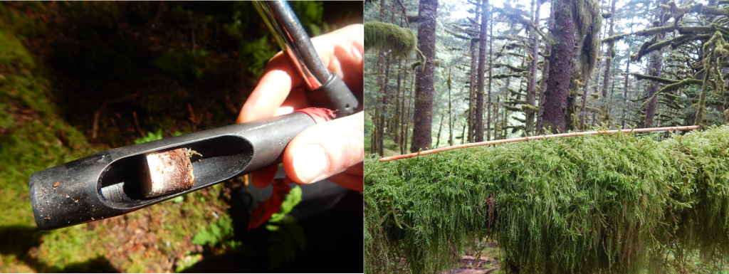
  4. From each tree, extract a few needles or bark disk for DNA extraction, and a tree core for age determination.

    A bark sample (there is a thin slice of multiplying cells in there) and a freshly extracted tree core

  5. Go find the next stand

    …before the loggers, if possible (these trees were standing two days earlier).

  6. Somewhere along this iterative process, pick up an additional, valuable team member.
DSCN6636

Hey Sally! Come get bushed with us!


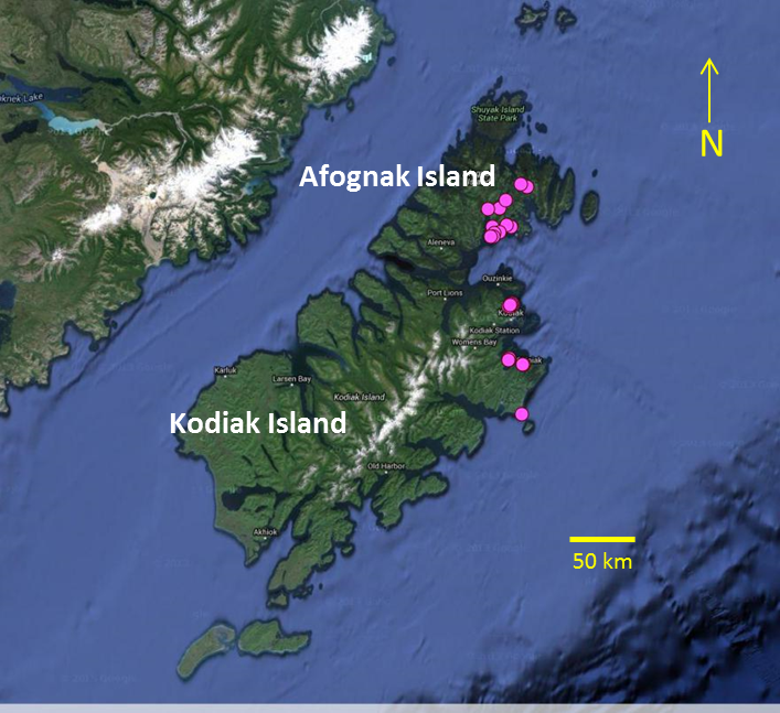
I ended up with a slightly structured distribution of stands (Mother Nature wasn’t told about the statistical advantages of spatial uniformity)…

kodiak_sample_map_full

Each pink dot is a sampled stand. (One pink dot might be hiding another)


…and occasionally, some fresh fish for dinner (thank you Ian)

Spot the beer… We’re so local.

By matching the age of sampled trees with their genotype across several stands , I will be able to directly monitor the evolution of the genetic makeup of the forest and answer the following questions:

How quickly do newly formed forests accumulate genetic diversity?

How many trees colonised the area, and from where?

Does relatedness among trees increase or decrease as we approach the front of expansion?


However, to properly answer these questions, I also need at least one “reference” Sitka spruce population that established a long time ago and can be considered to be in an equilibrium state in terms of genetic structure and diversity. The closest Sitka spruce forest that matches these requirements is on the Kenai Peninsula. That’s where the trip continues! Different landscapes, different challenges, different team, and so, very logically,…. different blogpost.


DSCN6538

To be continued…