Simulating climates in growth chambers – The AdapTree project
This post is part of the series Simulating Climates in Growth Chambers.
The AdapTree project evaluates the genetic and phenoptyic variation of two commercially important conifers in western Canada, interior spruce (Picea glauca, P. engelmannii, and their natural hybrids) and lodgepole pine (Pinus contorta). More than 580 seed sources were grown under controlled climate conditions to quantify genetic diversity and geographic structure for adaptive traits such as phenology, frost hardiness, seedling growth, and response to drought and heat. Concurrently, sequence capture and resequencing of much of the exome for ~600 individuals of each species reveals genetic variation, some of which is associated with this adaptation. Around 5,000 additional individuals per species growing in various other controlled climate regimes and outdoor common gardens will then be genotyped using a cheaper SNP array. All of these markers will be tested for a potential role in local adaptation to climate through 1) association with climate-relevant phenotypes; and 2) gene-environment correlations. The SNPs with evidence of local adaptation will then be used to evaluate the suitability of populations to future climates. Field-based validation studies have been established to confirm the genomic results.
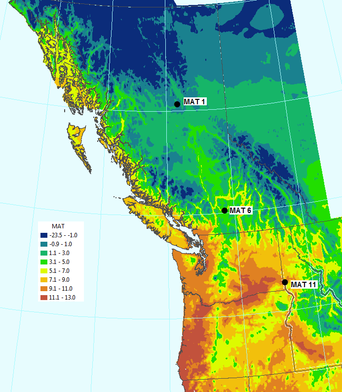
Location of the target simulated climates on a map.
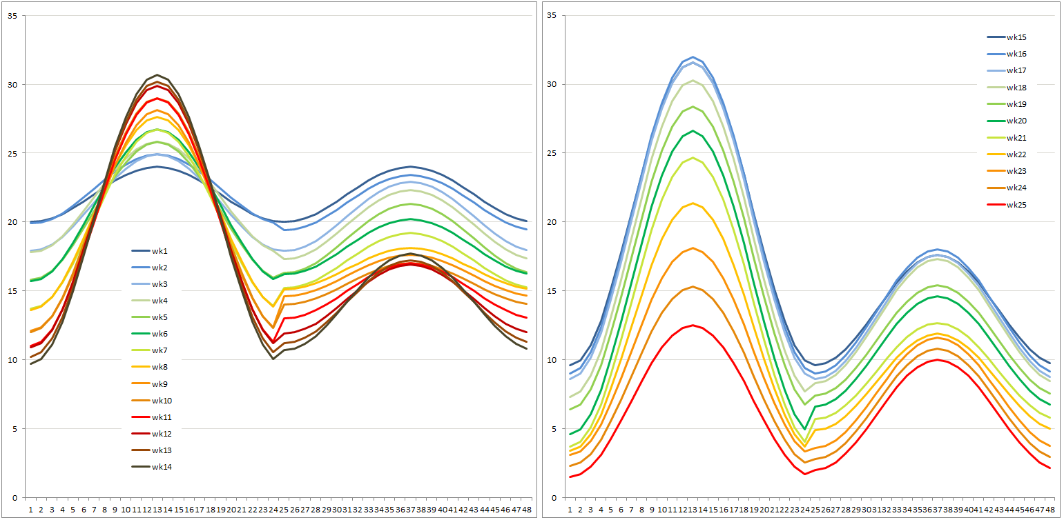
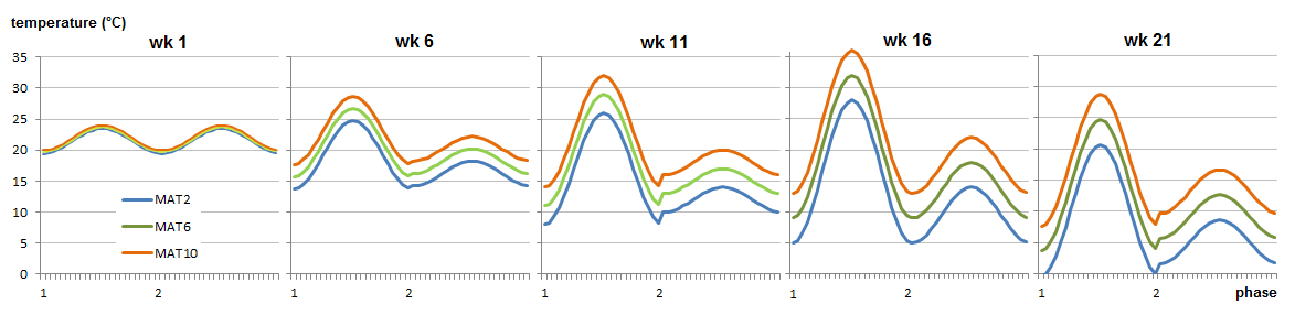
To bring out the differences in adaptive characteristics of populations from all over British Columbia and Alberta, three temperature regimes were developed to represent four different climates with mean annual temperatures (MAT) of 1, 6 and 11 °C (all well watered), as well as an MAT 11 dry climate.
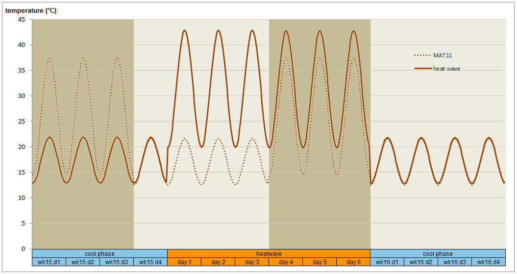
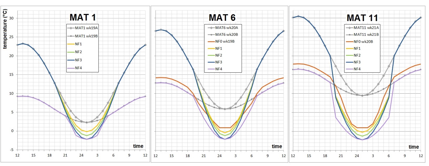
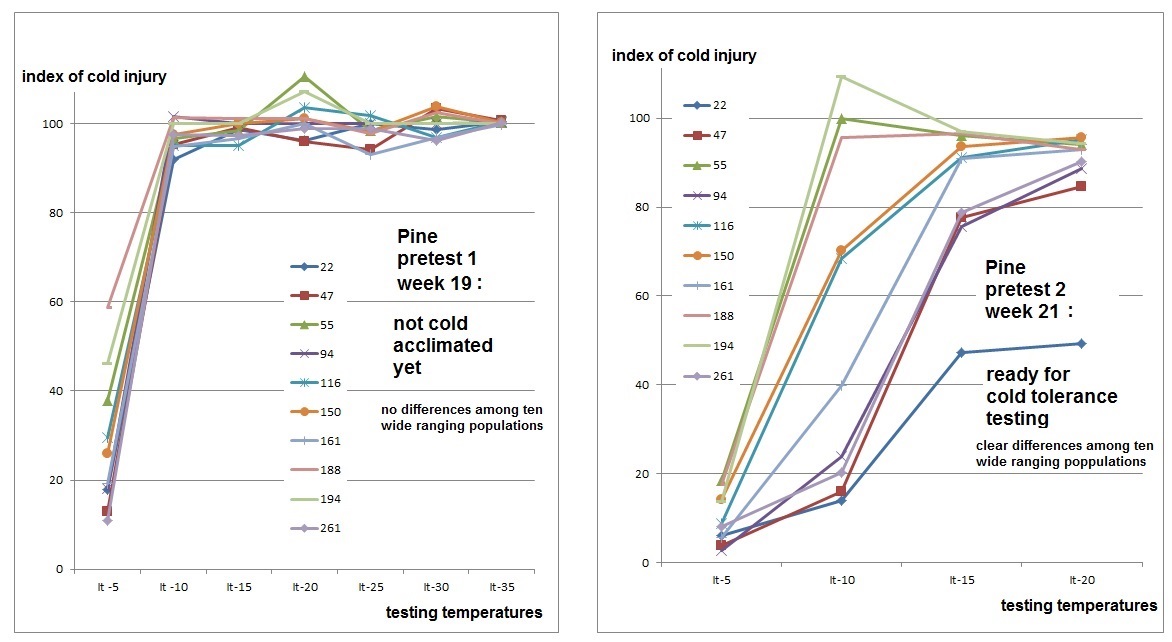
Realistic climates were needed to yield realistic bud break and bud set data in growth chambers. The photoperiod regime was identical for all plants and day length corresponds to that at 54.5°N at the relevant time of the season. Time constraints on the project necessitated germination modification and growing season compaction to reach the desired plant sizes quickly for all experiments. Not all experiments could be grown under fully controlled conditions, and some of the plants grown in the greenhouse were out of sync with nature yet needed to be planted outdoors in the following season. Their blackout regime gave us trouble, since covering them up to keep light out caused conditions ideal for fungal growth. During the second growing season, simulated drought was applied in cycles to the MAT11 dry treatment. Half of the plants in MAT11 wet and half of the plants in MAT11 dry were also subjected to a heat wave in the middle of summer. Plants were well-watered and chlorophyll fluorescence was measured to evaluate plant stress as a consequence of the heat wave. Carbon isotope composition was used to evaluate plant response to drought integrated over the growing season. At the end of the second growing season, cold hardiness measurements required us to simulate real winter, and not just a chilling period. The night frost pre-treatments were successful and good cold hardiness data were obtained. After this, the plants could be destructively sampled for dry weights. This required washing the soil off the roots. Thanks to our foresight in using plant cones during the first season (see root washing) we were able to separate the roots even for the largest (MAT 6 and 11) plants and after two seasons of growth.
Further information about the AdapTree project can be found on the website.