R Studio

PROCESS
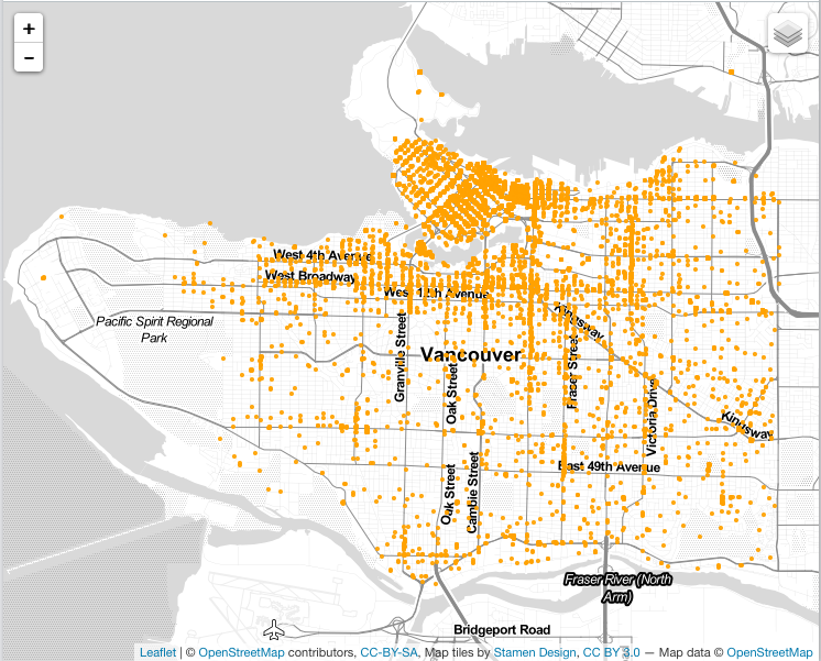
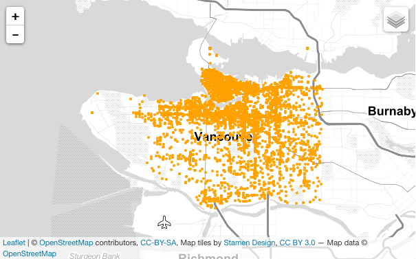
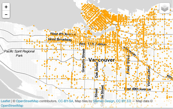
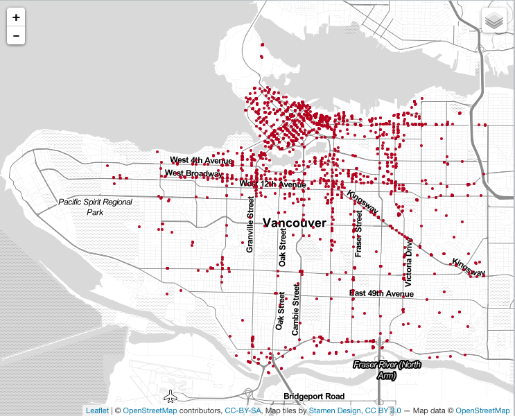
After parsing, geocoding, and filtering the data, 27275 out of 34354 records were retained.
VISUALIZATION
REFLECTION
A write up about your process and some insights from your visualization and a reflection on learning R and leaflet
Process:
You will need to demonstrate that you understand each step of the process of the data visualization pipeline as it relates to the work you’ve done. For each chunk of code that you’ve written, you will need to explain in writing on your blog what each step is doing – imagine if you needed to go step by step with your methods to the City of Vancouver Open Data Department, how would you document each step? This is in addition to commenting your code.
- After you finish creating the final data file to map, comment on: Understanding this data:
  1. Lost records of data: How many records did you start with? After running the data through parsing and geocoding and filtering, how many values did you end up with?
  2. Error: Do you think this is a lot or a little ‘error’? How reliable is this data?
  3. File formats: What is the difference between a shape (shp), csv, excel, geojson file. Which one did you create? Why? Given an example of when you would use each file.
Visualization:
Discuss the following. Be creative and thoughtful in your responses.
1. cartographic design: What are the cartographic constraints you encountered?
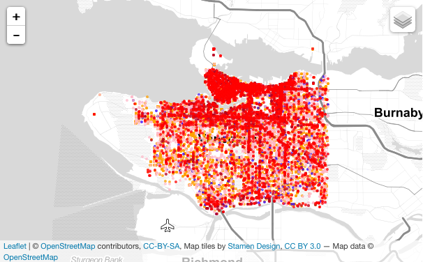
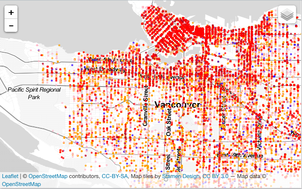
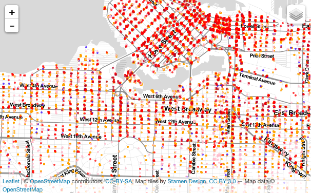
2. Discuss some insights you’ve found in your visualization upon using it: the spatial distribution, the types of crimes, what other data might be useful in this context, the interactivity – is it useful or not, etc?
Reflection
You have experience with expensive proprietary software packages ArcGIS and Adobe Illustrator that are supported by the UBC geography labs. Reflect on these few weeks of learning enough of an open source tool, R and leaflet, to create this interactive map. In your reflection discuss pros and cons of proprietary software and FOSS.

######################################################
# Vancouver Crime: Data Processing Script
# Date: October 30, 2016
# By: Annie Fang
# Desc: Vancouver Crime Data Visualization
######################################################

# ------------------------------------------------------------------ #
# ---------------------- Install Libraries ------------------------- #
# ------------------------------------------------------------------ #
install.packages("GISTools")
install.packages("RJSONIO")
install.packages("rgdal")
install.packages("RCurl")
install.packages("curl")

# Unused Libraries:
# install.packages("ggmap")
# library(ggmap)

# ------------------------------------------------------------------ #
# ----------------------- Load Libararies -------------------------- #
# ------------------------------------------------------------------ #
library(GISTools)
library(RJSONIO)
library(rgdal)
library(RCurl)
library(curl)

# ------------------------------------------------------------------ #
# ---------------------------- Acquire ----------------------------- #
# ------------------------------------------------------------------ #
# access from the interweb using "curl"
fname = curl('https://raw.githubusercontent.com/anniefangg/cartographiste/master/Crime2013.csv')

# Read data as csv
data = read.csv(fname, header=T)

# inspect your data
print(head(data))

# ------------------------------------------------- #
# -------------- Parse: Geocoder ------------------- #
# ------------------------------------------------- #
# change intersection to 00's
data$HUNDRED_BLOCK = gsub("X", "0", data$HUNDRED_BLOCK)
print(head(data$HUNDRED_BLOCK))

# Join the strings from each column together & add "Vancouver, BC":
data$full_address = paste(data$HUNDRED_BLOCK,
paste(data$STREET_NAME,
"Vancouver, BC",
sep=", "),
sep=" ")

# removing "Intersection " from the full_address entries
data$full_address = gsub("Intersection ", "", data$full_address)
print(head(data$full_address))

# a function taking a full address string, formatting it, and making
# a call to the BC government's geocoding API
bc_geocode = function(search){
# return a warning message if input is not a character string
if(!is.character(search)){stop("'search' must be a character string")}

# formatting characters that need to be escaped in the URL, ie:
# substituting spaces ' ' for '%20'.
search = RCurl::curlEscape(search)

# first portion of the API call URL
base_url = "http://apps.gov.bc.ca/pub/geocoder/addresses.json?addressString="

# constant end of the API call URL
url_tail = "&locationDescriptor=any&maxResults=1&interpolation=adaptive&echo=true&setBack=0&outputSRS=4326&minScore=1&provinceCode=BC"

# combining the URL segments into one string
final_url = paste0(base_url, search, url_tail)

# making the call to the geocoding API by getting the response from the URL
response = RCurl::getURL(final_url)

# parsing the JSON response into an R list
response_parsed = RJSONIO::fromJSON(response)

# if there are coordinates in the response, assign them to `geocoords`
if(length(response_parsed$features[[1]]$geometry[[3]]) > 0){
geocoords = list(lon = response_parsed$features[[1]]$geometry[[3]][1],
lat = response_parsed$features[[1]]$geometry[[3]][2])
}else{
geocoords = NA
}

# returns the `geocoords` object
return(geocoords)
}

# Geocode the events - we use the BC Government's geocoding API
# Create an empty vector for lat and lon coordinates
lat = c()
lon = c()

# loop through the addresses
for(i in 1:length(data$full_address)){
# store the address at index "i" as a character
address = data$full_address[i]
# append the latitude of the geocoded address to the lat vector
lat = c(lat, bc_geocode(address)$lat)
# append the longitude of the geocoded address to the lon vector
lon = c(lon, bc_geocode(address)$lon)
# at each iteration through the loop, print the coordinates - takes about 20 min.
print(paste("#", i, ", ", lat[i], lon[i], sep = ","))
}

# add the lat lon coordinates to the dataframe
data$lat = lat
data$lon = lon

# Write my file out
ofile = "/Users/anniefang/Desktop/GEOB_472/2013CaseLocationsDetails-Geo.csv"
write.csv(data, ofile)
# Find my geocoded dataset on GitHub: "https://raw.githubusercontent.com/anniefangg/cartographiste/CID/2013CaseLocationsDetails-Geo.csv"

# ------------------------------------------------- #
# --------------------- Mine ---------------------- #
# ------------------------------------------------- #
# --- Examine the unique cases --- #

# examine how the cases are grouped - are these intuitive?
unique(data$TYPE)

# examine the types of cases - can we make new groups that are more useful?
# Print each unique case on a new line for easier inspection
for (i in 1:length(unique(data$TYPE))){
print(unique(data$TYPE)[i], max.levels=0)
}

# Resulting 6 Groups
# [1] Other Theft
# [1] Break and Enter Residential/Other
# [1] Mischief
# [1] Theft of Vehicle
# [1] Theft from Vehicle
# [1] Break and Enter Commercial

# ------------------------------------------------- #
# --------------- Assign Vectors ------------------ #
# ------------------------------------------------- #

# Other Theft
Other_Theft = c('Other Theft')

# Break and Enter Residential/Other
Break_and_Enter_Residential_or_Other = c('Break and Enter Residential/Other')

# Mischief
Mischief = c('Mischief')

# Theft of Vehicle
Theft_of_Vehicle = c('Theft of Vehicle')

# Theft from Vehicle
Theft_from_Vehicle = c('Theft from Vehicle')

# Break and Enter Commercial
Break_and_Enter_Commercial = c('Break and Enter Commercial')

# ------------------------------------------------- #
# ------------------ Assign CID ------------------- #
# ------------------------------------------------- #

# give class id numbers:
data$cid = 9999
for(i in 1:length(data$TYPE)){
if(data$TYPE[i] %in% Other_Theft){
data$cid[i] = 1
}else if(data$TYPE[i] %in% Break_and_Enter_Residential_or_Other){
data$cid[i] = 2
}else if(data$TYPE[i] %in% Theft_of_Vehicle){
data$cid[i] = 3
}else if(data$TYPE[i] %in% Theft_from_Vehicle){
data$cid[i] = 4
}else if(data$TYPE[i] %in% Break_and_Enter_Commercial){
data$cid[i] = 5
}else{
data$cid[i] = 0
}
}

# --- handle overlapping points --- #
# Set offset for points in same location:
data$lat_offset = data$lat
data$lon_offset = data$lon

# Run loop - if value overlaps, offset it by a random number
for(i in 1:length(data$lat)){
if ( (data$lat_offset[i] %in% data$lat_offset) && (data$lon_offset[i] %in% data$lon_offset)){
data$lat_offset[i] = data$lat_offset[i] + runif(1, 0.0001, 0.0005)
data$lon_offset[i] = data$lon_offset[i] + runif(1, 0.0001, 0.0005)
}
}

# --- what are the top calls? --- #
# get a frequency distribution of the calls:
top_calls = data.frame(table(data$TYPE))
top_calls = top_calls[order(top_calls$Freq), ]
print(top_calls)

# Var1 Freq
# 6 Theft of Vehicle 840
# 1 Break and Enter Commercial 1758
# 2 Break and Enter Residential/Other 3008
# 3 Mischief 3715
# 5 Theft from Vehicle 7012
# 4 Other Theft 10942

# ------------------------------------------------------------------ #
# ---------------------------- Filter ------------------------------ #
# ------------------------------------------------------------------ #
# Filter data outside vancouver boundaries or an NA
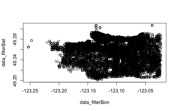
data_filter = subset(data, (lat <= 49.313162) & (lat >= 49.199554) &
(lon <= -123.019028) & (lon >= -123.271371) & is.na(lon) == FALSE )
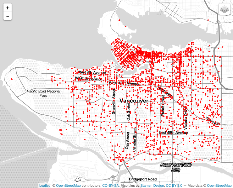
# plot the data
plot(data_filter$lon, data_filter$lat)

# Write out my file:
ofile_filtered = '/Users/anniefang/Desktop/GEOB_472/Crime2013-CID.csv'
write.csv(data_filter, ofile_filtered)

# Data set can also be found on GitHub: "https://raw.githubusercontent.com/anniefangg/cartographiste/CID/Crime2013-CID.csv"

# --- Convert Data to Shapefile --- #
# store coordinates in dataframe
coords_crime = data.frame(data_filter$lon_offset, data_filter$lat_offset)

# create spatialPointsDataFrame
data_shp = SpatialPointsDataFrame(coords = coords_crime, data = data_filter)

# set the projection to wgs84
projection_wgs84 = CRS("+proj=longlat +datum=WGS84")
proj4string(data_shp) = projection_wgs84

# set an output folder for our geojson files:
geofolder = "/Users/anniefang/Desktop/GEOB_472/"

# Join the folderpath to each file name:
opoints_shp = paste(geofolder, "crime_", "2013", ".shp", sep = "")
print(opoints_shp)
# File Name: '/Users/anniefang/Desktop/GEOB_472/crime_2013.shp'

opoints_geojson = paste(geofolder, "crime_", "2013", ".geojson", sep = "")
print(opoints_geojson)
# File Name: '/Users/anniefang/Desktop/GEOB_472/crime_2013.geojson'

# write the file to a shp
writeOGR(data_shp, opoints_shp, layer = "data_shp", driver = "ESRI Shapefile",
check_exists = FALSE)

# write file to geojson
writeOGR(data_shp, opoints_geojson, layer = "data_shp", driver = "GeoJSON",
check_exists = FALSE)

# ------------------------------------------------------------------ #
# ---------------------- Create Hexagon Grid ----------------------- #
# ------------------------------------------------------------------ #

# ------------------------ aggregate to a grid --------------------- #
# ref: http://www.inside-r.org/packages/cran/GISTools/docs/poly.counts
# set the file name - combine the shpfolder with the name of the grid
grid_fn = '/Users/anniefang/Desktop/GEOB_472/hexagonfiles/grid_fn.txt'

# read in the hex grid setting the projection to utm10n
hexgrid = readOGR(grid_fn, 'OGRGeoJSON')

# OGR data source with driver: GeoJSON
# Source: "/Users/anniefang/Desktop/GEOB_472/hexagonfiles/grid_fn.txt", layer: "OGRGeoJSON"
# with 5104 features
# It has 4 fields

# transform the projection to wgs84 to match the point file and store it to a new variable (see variable: projection_wgs84)
hexgrid_wgs84 = spTransform(hexgrid, projection_wgs84)

# ------------------------------------------------------------------ #
# ------------------ Assign Values to Hexagons --------------------- #
# ------------------------------------------------------------------ #

# Use the poly.counts() function to count the number of occurrences of calls per grid cell
grid_cnt = poly.counts(data_shp, hexgrid_wgs84)

# define the output names:
ohex_shp = paste(geofolder, "hexgrid_250m_", "Crime2013", "_cnts",
".shp", sep = "")
print(ohex_shp)
# Output Name File: '/Users/anniefang/Desktop/GEOB_472/hexgrid_250m_Crime2013_cnts.shp'

ohex_geojson = paste(geofolder, "hexgrid_250m_","Crime2013","_cnts",".geojson")
print(ohex_geojson)
# Output Name File: '/Users/anniefang/Desktop/GEOB_472/ hexgrid_250m_ Crime2013 _cnts .geojson'

# write the file to a shp
writeOGR(check_exists = FALSE, hexgrid_wgs84, ohex_shp,
layer = "hexgrid_wgs84", driver = "ESRI Shapefile")

# write file to geojson
writeOGR(check_exists = FALSE, hexgrid_wgs84, ohex_geojson,
layer = "hexgrid_wgs84", driver = "GeoJSON")

# ------------------------------------------------------------------ #
# --------------------- END DATA PROCESSING ------------------------ #
# ------------------------------------------------------------------ #

######################################################
# Vancouver Crime: Leaflet Script
# Date: October 30, 2016
# By: Annie Fang
# Desc: Vancouver Crime Data Visualization
######################################################

# ------------------------------------------------------------------ #
# -------------------- Install Leaflet Library --------------------- #
# ------------------------------------------------------------------ #

# install the leaflet library
install.packages("leaflet")

# add the leaflet library to your script
library(leaflet)

# initiate the leaflet instance and store it to a variable
m = leaflet()

# we want to add map tiles so we use the addTiles() function - the default is openstreetmap
m = addTiles(m)

# we can add markers by using the addMarkers() function
m = addMarkers(m, lng=-123.256168, lat=49.266063, popup="T")

# we can "run"/compile the map, by running the printing it
m

# ------------------------------------------------------------------ #
# -------------------- Working With Point Data --------------------- #
# ------------------------------------------------------------------ #

filename = "/Users/anniefang/Desktop/GEOB_472/Crime2013-CID.csv"
data_filter = read.csv(filename, header = TRUE)

# Data on GitHub Provided:
# data_filter = read.csv(curl('https://raw.githubusercontent.com/anniefangg/cartographiste/CID/Crime2013-CID.csv'), header=TRUE)

# subset out your data_filter:
df_Other_Theft = subset(data_filter, cid == 1)
df_Break_and_Enter_Residential_or_Other = subset(data_filter, cid == 2)
df_Mischief = subset(data_filter, cid == 3)
df_Theft_of_Vehicle = subset(data_filter, cid == 4)
df_Theft_from_Vehicle = subset(data_filter, cid == 5)
df_Break_and_Enter_Commercial = subset(data_filter, cid == 0)

# ------------------------------------------------------------------ #
# -------------------- Initiate Base Map Tiles --------------------- #
# ------------------------------------------------------------------ #

# initiate leaflet
m = leaflet()

# add openstreetmap tiles (default)
m = addTiles(m)

# you can now see that our maptiles are rendered
m

# ------------------------------------------------------------------ #
# --------------- Define Symbology for Point Layers ---------------- #
# ------------------------------------------------------------------ #

colorFactors = colorFactor(c('red', 'orange', 'purple', 'blue', 'pink', 'brown'),
domain = data_filter$cid)
# Other_Theft
m = addCircleMarkers(m,
lng = df_Other_Theft$lon_offset,
lat = df_Other_Theft$lat_offset,
popup = df_Other_Theft$Case_Type,
radius = 2,
stroke = FALSE,
fillOpacity = 0.75,
color = colorFactors(df_Other_Theft$cid),
group = "1 - Other Theft")

# Break_and_Enter_Residential_or_Other
m = addCircleMarkers(m,
lng = df_Break_and_Enter_Residential_or_Other$lon_offset,
lat = df_Break_and_Enter_Residential_or_Other$lat_offset,
popup = df_Break_and_Enter_Residential_or_Other$Case_Type,
radius = 2,
stroke = FALSE,
fillOpacity = 0.75,
color = colorFactors(df_Other_Theft$cid),
group = "2 - Break and Enter Residential or Other")

# Mischief
m = addCircleMarkers(m,
lng = df_Mischief$lon_offset,
lat = df_Mischief$lat_offset,
popup = df_Mischief$Case_Type,
radius = 2,
stroke = FALSE,
fillOpacity = 0.75,
color = colorFactors(df_Mischief$cid),
group = "3 - Mischief")

# Theft_of_Vehicle
m = addCircleMarkers(m,
lng = df_Theft_of_Vehicle$lon_offset,
lat = df_Theft_of_Vehicle$lat_offset,
popup = df_Theft_of_Vehicle$Case_Type,
radius = 2,
stroke = FALSE,
fillOpacity = 0.75,
color = colorFactors(df_Theft_of_Vehicle$cid),
group = "4 - Theft of Vehicle")

# Theft_from_Vehicle
m = addCircleMarkers(m,
lng = df_Theft_from_Vehicle$lon_offset,
lat = df_Theft_from_Vehicle$lat_offset,
popup = df_Theft_from_Vehicle$Case_Type,
radius = 2,
stroke = FALSE,
fillOpacity = 0.75,
color = colorFactors(df_Theft_from_Vehicle$cid),
group = "5 - Theft from Vehicle")

# Break_and_Enter_Commercial
m = addCircleMarkers(m,
lng = df_Break_and_Enter_Commercial$lon_offset,
lat = df_Break_and_Enter_Commercial$lat_offset,
popup = df_Break_and_Enter_Commercial$Case_Type,
radius = 2,
stroke = FALSE,
fillOpacity = 0.75,
color = colorFactors(df_Break_and_Enter_Commercial$cid),
group = "0 - Break and Enter Commercial")

# ------------------------------------------------------------------ #
# ------------------- Additional Base Map Tiles -------------------- #
# ------------------------------------------------------------------ #

m = addTiles(m, group = "OSM (default)")
m = addProviderTiles(m,"Stamen.Toner", group = "Toner")
m = addProviderTiles(m, "Stamen.TonerLite", group = "Toner Lite")

m = addLayersControl(m,
baseGroups = c("Toner Lite","Toner"),
overlayGroups = c("1 - Other Theft", "2 - Break and Enter Residential or Other",
"3 - Mischief","4 - Theft of Vehicle", "5 - Theft from Vehicle",
"0 - Break and Enter Commercial")
)

# make the map
m

# ------------------------------------------------------------------ #
# ----------------------------- Toggle ----------------------------- #
# ------------------------------------------------------------------ #

# Put variables into a list to loop:
data_filterlist = list(df_Other_Theft = subset(data_filter, cid == 1),
df_Break_and_Enter_Residential_or_Other = subset(data_filter, cid == 2),
df_Mischief = subset(data_filter, cid == 3),
df_Theft_of_Vehicle = subset(data_filter, cid == 4),
df_Theft_from_Vehicle = subset(data_filter, cid == 5),
df_Break_and_Enter_Commercial = subset(data_filter, cid == 0))

# List of Layers:
layerlist = c("1 - Other Theft", "2 - Break and Enter Residential or Other",
"3 - Mischief","4 - Theft of Vehicle", "5 - Theft from Vehicle",
"0 - Break and Enter Commercial")

# Same color variable:
colorFactors = colorFactor(c('red', 'orange', 'purple', 'blue', 'pink', 'brown'), domain=data_filter$cid)

# Loop - add markers to the map object:
for (i in 1:length(data_filterlist)){
m = addCircleMarkers(m,
lng=data_filterlist[[i]]$lon_offset,
lat=data_filterlist[[i]]$lat_offset,
popup=data_filterlist[[i]]$Case_Type,
radius=2,
stroke = FALSE,
fillOpacity = 0.75,
color = colorFactors(data_filterlist[[i]]$cid),
group = layerlist[i]
)
}

# ------------------------------------------------------------------ #
# ------------------- Radiobutton Functionality -------------------- #
# ------------------------------------------------------------------ #

m = addTiles(m, "Stamen.TonerLite", group = "Toner Lite")
m = addLayersControl(m,
overlayGroups = c("Toner Lite"),
baseGroups = layerlist
)
m

# ------------------------------------------------------------------ #
# ---------------- Aggregate Data to Hexagonal Grid ---------------- #
# ------------------------------------------------------------------ #

library(rgdal)
library(GISTools)

# define the filepath
hex_crime_fn = '/Users/anniefang/Desktop/GEOB_472/hexgrid_250m_Crime2013_cnts.geojson'

# read in the geojson
hex_crime = readOGR(hex_crime_fn, "OGRGeoJSON")

# OGR data source with driver: GeoJSON
# Source: "https://raw.githubusercontent.com/anniefangg/cartographiste/Hexgrid-Crime2013-geojson/%20hexgrid_250m_%20Crime2013%20_cnts%20.geojson", layer: "OGRGeoJSON"
# with 5104 features
# It has 4 fields

# Stamen Toner Lite Style
m = leaflet()
m = addProviderTiles(m, "Stamen.TonerLite", group = "Toner Lite")

# Create a continuous palette function
pal = colorNumeric(
palette = "Greens",
domain = hex_crime$data
)

# add the polygons to the map
m = addPolygons(m,
data = hex_crime,
stroke = FALSE,
smoothFactor = 0.2,
fillOpacity = 1,
color = ~pal(hex_crime$data),
popup = paste("Number of calls: ", hex_crime$data, sep="")
)

# Add legend
m = addLegend(m, "bottomright", pal = pal, values = hex_crime$data,
title = "Vancouver Crime Density 2013",
labFormat = labelFormat(prefix = " "),
opacity = 0.75
)

m

# initiate leaflet map layer
m = leaflet()
m = addProviderTiles(m, "Stamen.TonerLite", group = "Toner Lite")

# --- hex grid --- #
# store the file name of the geojson hex grid
hex_crime_fn = '/Users/anniefang/Desktop/GEOB_472/hexgrid_250m_Crime2013_cnts.geojson'

# read in the data
hex_crime = readOGR(hex_crime_fn, "OGRGeoJSON")

# Create a continuous palette function
pal = colorNumeric(
palette = "Greens",
domain = hex_crime$data
)

# add hex grid
m = addPolygons(m,
data = hex_crime,
stroke = FALSE,
smoothFactor = 0.2,
fillOpacity = 1,
color = ~pal(hex_crime$data),
popup= paste("Number of calls: ",hex_crime$data, sep=""),
group = "hex"
)

# add legend
m = addLegend(m, "bottomright", pal = pal, values = hex_crime$data,
title = "Vancouver Crime Density 2013",
labFormat = labelFormat(prefix = " "),
opacity = 0.75
)

# --- points data --- #

# subset out your data:
df_Other_Theft = subset(data_filter, cid == 1)
df_Break_and_Enter_Residential_or_Other = subset(data_filter, cid == 2)
df_Mischief = subset(data_filter, cid == 3)
df_Theft_of_Vehicle = subset(data_filter, cid == 4)
df_Theft_from_Vehicle = subset(data_filter, cid == 5)
df_Break_and_Enter_Commercial = subset(data_filter, cid == 0)

data_filterlist = list(df_Other_Theft = subset(data_filter, cid == 1),
df_Break_and_Enter_Residential_or_Other = subset(data_filter, cid == 2),
df_Mischief = subset(data_filter, cid == 3),
df_Theft_of_Vehicle = subset(data_filter, cid == 4),
df_Theft_from_Vehicle = subset(data_filter, cid == 5),
df_Break_and_Enter_Commercial = subset(data_filter, cid == 0))
# List of Layers:
layerlist = c("1 - Other Theft", "2 - Break and Enter Residential or Other",
"3 - Mischief","4 - Theft of Vehicle", "5 - Theft from Vehicle",
"0 - Break and Enter Commercial")

colorFactors = colorFactor(c('red', 'orange', 'purple', 'blue', 'pink', 'brown'), domain=data_filter$cid)
for (i in 1:length(data_filterlist)){
m = addCircleMarkers(m,
lng=data_filterlist[[i]]$lon_offset, lat=data_filterlist[[i]]$lat_offset,
popup=data_filterlist[[i]]$Case_Type,
radius=2,
stroke = FALSE, fillOpacity = 0.75,
color = colorFactors(data_filterlist[[i]]$cid),
group = layerlist[i]
)

}

m = addLayersControl(m,
overlayGroups = c("Toner Lite", "hex"),
baseGroups = layerlist
)

# show map
m