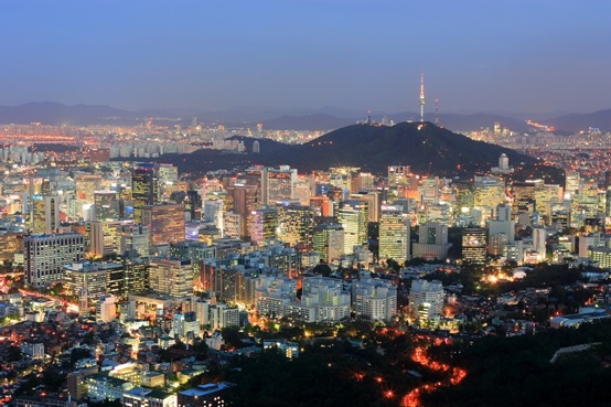
The greenbelt in Seoul
What greenbelt is
Land use planning policy, firstly introduced in UK, is explicitly encourages urban densification by restricting land for several purposes such as for environment and natural resources protection and urban sprawl prevention.[1]
Background and the Policy origin
Seoul is a central city of Seoul Metropolitan Area including Seoul, Incheon and Gyeonggi.[2][5]From 1950 to 1975, the growth of Seoul was rapid at annual rate of 7.6 percent, on average.[3] Seoul’s population in 1975 was about 7 times higher than in 1950; a million in 1950 and 6.8 million in 1975.[3] The Capital Region Urban plan was proposed by the Korean Planners Association in 1963.[4] The plan included designing the greenbelt within satellite towns along the corridor between Seoul and Incheon in Korea.[4] Under the Town Planning Act, the greenbelt was created and introduced in Korea in1971; however, the greenbelt was formally defined as “Development Restriction Zone”.[4] The greenbelt also played an important role in National Comprehensive Physical Plan of 1972-1981.[4] With an intervention of President Jung Hee Park, Seoul government firstly implemented the greenbelt to Seoul in July 1971.[4] Since two years after 1971, the greenbelt was built in 13 cities including Busan, Daegu, Kwangju and Daejeon.[3] Yeocheon became the last city implementing this policy in 1977.[3] Seoul metropolitan area reformed the greenbelt in 1990[5]; however, this posting is focused on pre-existing greenbelt before the reform.

Objectives
There are seven objectives of this policy:[3][4]
1) To ease the rapid growth rate of population and to prevent industrial concentration in Seoul[4]
2) To restrict expansion of Seoul into neighbour cities such as Incheon, Suwon and Euijeongbu[4]
3) To restrict expansion to the north near to North Korea for national security[4]
4) To reserve the land for environmental purpose [4]
5) To prevent the formation illegal suburban around Seoul[3]
6) To protect land for agricultural use[3]
7) To balance the growth of Seoul and suburban cities like Incheon[3]
Implementation
The paper, ” KOREA’S GREENBELTS: IMPACTS AND OPTIONS FOR CHANGE”, described the development of the greenbelt in Seoul metropolitan area in following four phases:
1) The Greenbelt was located 15 kilometres (km) away from City Hall. As the north-west area is near to north Korea, it was also included in greenbelt zone for national defence. The total area encircled by the belt was 463.8 square kilometres (km2).[3]
2) 86.8km2 were added to the existing greenbelt zone as the greenbelt was extended to include Anyang, suburban surrounding Seoul, to protect its environment.[3]
3) The width of the belt was extended from 15 to 35 km. The total greenbelt zone increased to 768.6 km2 by extending the belt to the land located in eastern side of Han River.[3]
4) With including Ansan, a new town in the southwest of Seoul metropolitan area, the area encircled by the greenbelt was increased by 247.6 km2.[3]The total area within the belt was 1566.8 km2 and its width became 40 km.[3]Seoul had 153 km2 within the greenbelt.[5]
Coverage
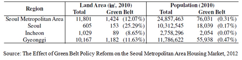
Total area in Seoul Metropolitan Area covered by the greenbelt was 1566.8 km2 in 1980s; however, it was decreased to 1424 km2 in 2010 data due to the greenbelt reform in 1990.[3][5]Seoul has had 153 km2 area within the greenbelt.[5] This land area is about 1.3% (=153/11801) of total land area in Seoul Metropolitan area. The greenbelt, the policy encouraged urban densification was employed in both central city and suburb of the Seoul metropolitan area. But, this blog is focuesed on Seoul, the central city of metropolitan area. Base on 2010 data given in the following table, 18,039 people lived within Seoul greenbelt. The population covered by Seoul greenbelt was about 0.07% (=18039/24857463) of the total population of the Seoul Metropolitan Area.[5] 0.008% of the metropolitan area population was covered by Incheon greenbelt and 0.23% was covered by belt in Gyeonggi.
Effectiveness
I found two papers including the content related to the effectiveness of the Seoul greenbelt: KOREA’S GREENBELTS: IMPACTS AND OPTIONS FOR CHANGE and SEOUL’S GREENBELT:AN EXPERIMENT IN URBAN CONTAINMENT. As the authors of these papers noted, there are no actual evaluation done to prove its effectiveness and only few suggestions for its measurement were done by researchers. To measure the effectiveness, calculation of social costs and social benefits of the greenbelt comparison are necessary. If the benefits outweigh the costs, the greenbelt’s effectiveness can be proven.[3] Bae (1998) described three categories of benefit from the implementation of the greenbelt in Seoul: (1) amenity value of the land within the greenbelt, (2) the government’s savings due to efficiently compacted development of public services such as a public transport, (3) value of ecosystem and environmental quality. The greenbelt’s social costs are incurred from higher prices of land and housing, and an increase in commuting expense and infrastructure spending. According to her estimation, high travel expense was a key component to increase the social cost. Annual travel cost per individual was about 250,000 Won (₩) and the social costs were ₩ 470 billion.[3]In 1987, the values of greenbelt land were 30 percent lower than non-greenbelt land values.[4] With an assumption that Seoul completely eliminated the greenbelt in 1987, greenbelt land values would be increased by 32.1 percent while non-greenbelt values would be declined by 7.5 percent.[4] High benefits were estimated as the amenity value of the greenbelt land was significant and people were willing to protect land for future generation.[3] However, these benefits were not enough to outweigh social costs incurred from the skyrocketing non-greenbelt land and housing price due to a rapid population growth in Seoul.[3]
Distributional Effect
Based on my research, the impact of the greenbelt on people is different depending on people’s income level and where they live:
(1) a negative impact on the poor living in the non-greenbelt
(2) a negative impact on the rich living in the greenbelt
(3) a positive impact on rich people in the non-greenbelt.
As Seoul became one of the cities with high density due to a rapid population growth and the greenbelt, the greenbelt land and housing price was lower than non-greenbelt. The price of non-greenbelt area skyrocketed due to excess demand. Poor people living in non-greenbelt land could not afford a high housing price while the rich having housing ownership could earn benefits. As 80% of the greenbelt land was owned by rich people, they were more negatively affected by low housing price. However, a negative impact on the rich living in the greenbelt can be cancelled by a positive impact on the rich living in the non-greenbelt. Therefore, I can conclude that poor people are more impacted by the greenbelt.
Conclusion
Seoul greenbelt was successful to encourage densification. Due to the greenbelt and population growth, land supply was restricted to satisfy high demand and Seoul became one of the highest density city. However, I don’t think that the policy is efficient at all. Skyrocketing housing price can cause bigger economic gap between people with different income level and greater dissatisfaction of residents in Seoul with the government. I believe that Seoul should eliminate the greenbelt except a few areas for the national defence and environment protection.
Reference
[1] http://en.wikipedia.org/wiki/Green_belt
2] https://en.wikipedia.org/wiki/Seoul_Capital_Area
[3] http://digital.law.washington.edu/dspace-law/bitstream/handle/1773.1/867
/7PacRimLPolyJ479.pdf?sequence=1
[4] http://www.nrs.fs.fed.us/pubs/gtr/gtr_nc265/gtr_nc265_027.pdf
[5] http://smartgrowth.umd.edu/assets/documents/acsp/acsp2012pres_jeon.pdf