Please note: the source for this material is from the lab instructions and my own lab results/write up, unless otherwise stated
PDFs of all the maps can be found here.
Lab 1 – Spatial Stats Using Modelbuilder Tutorial
In this lab, the techniques surrounding the use of Modelbuilder were introduced and explored. The steps in this lab were: 1) download data from the Centres for Disease Control, 2) Join this data into a geodatabase in ArcMap 3) Create a model so that individual feature classes can be made 4) create a model for hotspot analysis 5) use the animation tool to see the changes in the hotspots over the years. A technique that was unique to this lab was adding a prefix of “0” to all the raw CountyCodes data in Excel such that, the join into ArcMap would work smoothly.
Using techniques surrounding the concepts of data retrieval, geodatabase creation, numbers and text, features, modeling building, and animation, this map shows the hotspot and coldspot areas within the Southern United States of America that have reported cases of heart disease rate. Maps were generated for 18 years, from 1999 to 2016. The animation tool showed the changes and progression of hot and cold spots throughout the years, allowing the identification of patterns. Most years had mainly hotspots, without evident coldspots, and all maps had a majority of insignificant areas (ie. Neither a hotspot nor a coldspot).
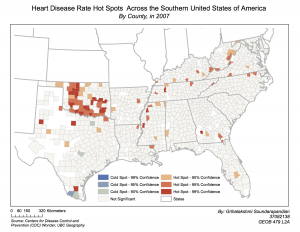
This particular maps shows the distribution in year 2007. We can see that a majority of the hotspots, or areas of greater heart disease, dominate the northwest portion of the study area, creating a clustered pattern. Hotspot areas between 90% and 99% confidence all reside here. This infers that this area is at highest risk for heart disease – a collective health issue in this area.
LAB 2 – EXPLORING FRAGSTATS
Fragstats is a software that calculates the existence of various landscape metrics, enabling a user to detect change in landscape and land use across an area over time (Fragstats, 2000). Using Fragstats, this lab explored the change in landuse in Edmonton over a ten year span, between 1966-1976, and a transition matrix was created to analyze the transition of land use from one use to another across the time period. From the hypothetical standpoint of a consultant working for the City of Edmonton, these results were shared and interpreted within a written report.
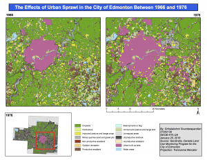
Map 1. The final map showing the land use changes in Edmonton between 1966 and 1976
Sustainable living and infrastructure has become a key component to urban development over the last few decades. As climate change impacts become a reality, harming all aspects of the environment, it is the responsibility of municipalities to ensure that future urban development protects as much cropland, natural forests, as bogs as possible. Analysis of land use changes within the city of Edmonton between 1966 to 1976, using land use data for Edmonton from the Canada Land Use Monitoring Program (CLUMP) to conduct spatial analysis via ArcMap and Fragstats, show that 4.2% of cropland was converted into urban development, as displayed in the map above and the tables below. This creates the problem of urban sprawl, and resulting in deforestation, loss of prime cropland, and various health and socioeconomic consequences. Hence, we recommend that the City of Edmonton take a conservative approach and create a 500m land buffer around forests and cropland that border future urban development, alongside implementation of forest reserves. This will lower environmental impacts, and create an awareness of the importance of natural environments and farmland, aiding the City of Edmonton in reaching its 10 sustainability goals (Edmonton, 2018) to build a city of resilience and green living.
Table 1. Fragstat Metrics describing the various class and landscape metrics for all the landuse types between 1966 and 1976
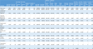
Table 2. Transition Matrix of Landuse Changes between 1966 and 1976. Includes percent change – the overall change in each land use over the time frame. 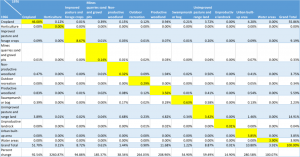
LAB 3 – INTRODUCTION TO GEOGRAPHICALLY WEIGHTED REGRESSION
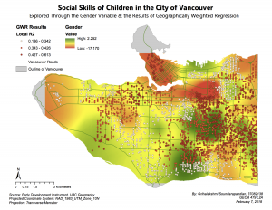
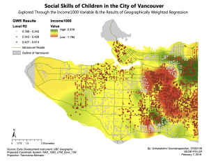
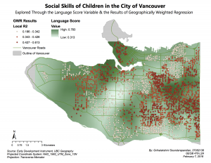
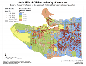
In conjunction with our lecture about statistics and regression, this lab focused on using Geographically Weighted Regression to analyze the influence of a set of individual and neighbourhood characteristics/variables (ex. family income, language and physical abilities of the child, etc.) on the social skills of children, and comparing these results to that of the Ordinary Least Squares method using with the same data. GWR allowed the recognition of local relationships between the variables, and this produced meaningful results, whereas the OLS generated more global results. This lab provided an opportunity to use the ‘Modelling Spatial Relations’ toolbox in ArcMap, and particularly the explanatory regression analysis tool. This enabled us to explore the use of independent and dependent variables and produce a set of ‘most important’ variables to use within the GWR analysis. The variables of focus for the GWR analysis were language, gender, and income, and a grouping analysis was conducted to interpret the results of the GWR and the OLS. The results of this lab are as follows:
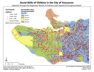
The full write up for this lab can be found here.
LAB 4 – INTRODUCTION TO CRIMESTAT
In accordance with the lecture exploring the use of GIS in crime analysis, lab 4 used the software of CrimeStats to investigate the distribution of crimes such as residential and commercial break and enters, robberies, and car thefts, within the Ottawa-Nepean area. This lab was assigned in order to provide us practice with analysis how a change in baseline population affects the data, and how different methods of data analysis can render similar or different results. Within this lab, we explored various methods to identify clustering within the crimes. These methods were: nearest neighbour statistics, spatial autocorrelation hotspots, fuzzy mode analysis, spatial-temporal hotspots (to see if the crimes are clustered in both time and space), and single and dual surface kernel density interpolation (to gather a broad understanding of the crime distribution). The results of these analyses and their comparisons can be found below:
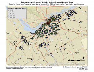
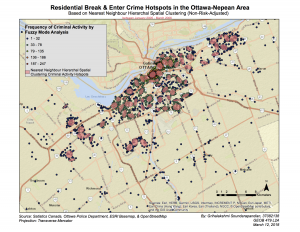
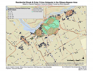
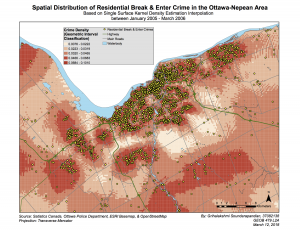
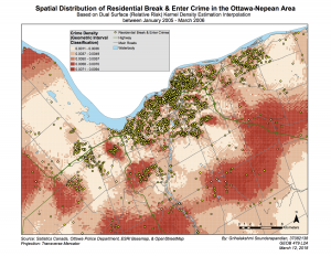
The full write up for this lab, including comparisons of all the results, can be found here.