03/7/18

The Homebrew Series: Inferring demographic history with ABC, by Joane Elleouet and Sally Aitken

Want to know about the history of the populations you’re studying? Joane Elleouet and Sally Aitken see how far Approximate Bayesian Computation (ABC) and your sequencing method of choice can take you in a new paper in Molecular Ecology Resources.

20 years ago, Tavaré et al. used ABC to estimate that the time to coalescence for the human population based on the Y chromosome was about 157,300 years ago (but!) and evolutionary biologists were off to the races. Now ABC is a common tool in the field with many software implementations to choose from. A lot else has happened in the last 20 years – like huge advances in genotyping technology. Even for non-model species, we can now get lots of genomic data for cheaper than ever using reduced representation library sequencing methods like genotyping-by-sequencing and GBS.

But how well does ABC perform with RRL data and different demographic models? What are its limitations? How do you make the best choices for your sequencing efforts? To answer these questions, Jo simulated data sets for 4 kinds of demographic models and 5 types of sequencing efforts and performed ABC on those datasets. She compared different model’s performance with

  • phased and unphased data, (phasing doesn’t help)
  • data from lots of short reads vs fewer, longer sequences (lots of short reads just as good)
  • different times since colonization, (depends on parameter value and demographic model)
  • tradeoffs between number and individuals and sampling depth at different sequencing error rates, (go for more individuals over depth)
  • and compared ABC to an SFS method. (similar)

As far as the different demographic models they consider, they find that ABC can be used with data from reduced representation library sequencing methods to precisely infer very simple demographic models, but not complex ones.

Here’s what Aitken Lab members had to say after reading the paper:

What’s your takeaway from this paper?

Reader 1: This paper provides several rules of thumb for inferring demographic events from incomplete, fragmented genomic data. Demographic models should be kept as simple as possible, and numerous short sequences from many individuals is preferable to fewer long sequences from a small sample of the population.

Reader 2: You’d better know what kind of demographic history your population has before you start trying to estimate parameters!

Reader 3: Estimating demographic parameters with ABC has limitations even with very simple demographic models

What’s the coolest thing about this paper?

R1: Improving techniques to infer the ancient demographic history of any species you like, not just model species.

R2: I didn’t realize how hard inferring demographic history is, even with so much genomic data. The extensive simulations are really impressive and convincing.

R3: Adding a realistic component by testing the effect of sequencing depth and error

What questions are you left with after reading this paper?

R2: How often do researchers know the “right” model of demographic history to try to infer? Whether or not to include migration or how many populations there have been? How do people figure this out?

R3: What if summary statistics lead to a too drastic loss of data? is there a better way to summarize the data while keeping crucial information?

 

01/28/18

The Homebrew series: Novel climates in BC, by Colin Mahony et al.

The year got off to a flying start in the Aitken lab, with a Forest Ecology and Management publication from our own Colin Mahony and his collaborators. Basically, if everyone else’s year started on a rocket, it’d better be running on clean energy. Following on his recent Global Change Biology publication, Colin shows us that human induced climate change is no joke to our beloved BC forests, and the future might be more grim than previously anticipated by forest managers. Colin shows that novel climates, climates that are currently not experienced anywhere in BC, might arise in BC by mid-century, and that these unprecedented conditions may fall under the radar with the current use of the BEC projection model.

At the moment, the best way to decide what forest tree species to plant where is to project ourselves forward about 50 years (about the time it takes for forestry trees to become fully mature) and determine what climate will be occurring then in the area of interest. Tree species and provenances can then be selected from BC areas with the closest contemporary climate. This is all done through the BEC system, which groups BC climatic conditions in an ecologically meaningful set of units.

The crucial question is: what if there is no place in BC that matches the predicted future climate of an area? Should we expand our range to all of North America? Well, Colin et al. actually show that some mid-century novel climates of BC have no equivalent in other parts of North America either…

These results highlight the limitations of the BEC projection model: 2 of the measures of the method, analog similarity and ensemble agreement, are actually diagnostic of novel climates at high values. In other words, projections of future BEC climates can be erroneous in novel climates, in particular by creating an appearance of reduced climate disruption and uncertainty. In providing a map of where novel climates are likely, this research points to regions where BEC projections are reliable from areas where other analytical approaches are required.

Here’s what lab members reading the paper had to say about it:

What’s our takeaway from this paper?

We don’t know what we think we know about future climate/ecology predictions in lowlands, coastal regions, and NE BC, because the climates there are unlike all others in North America. Forest management practices should rely on a species-specific basis, and be adapted with new management approaches—not found in other BEC zones’ practices.

“The best match is not necessarily a good match.” Depending on the analog pool, amount of climate change, and particular decision framework you use, you may find that the best climate analog is nothing like the actual climate. If I’m picking my pants from the kids section, the biggest ones are the best fit, but I can still only get one leg in them!

What’s the coolest thing about this paper?

Standardizing changes in climate by interannual variablility is a really cool way of expressing their ecological relevance, and if you want to know more about this smart method, check out Mahony et al. 2017. Also, despite the uncertainties in predicting the future of ecosystems under climate change, this study presents a fine-scale adjustment on what was known and on what was expected for British Columbian forests under climate change. The provided information will be key to reducing the risks of resource losses in the province.

Figures 2 and 3 are such awesome figures. They clearly and concisely explain a concept that can be difficult to get your head around.

What question are we left with after reading this paper?

What would the scenario of novel climates be on a global scale using the same approach?

What management methods should we use in areas where novel climates are predicted to occur?

Is Colin’s middle name Reginald? Rudolphus? Royce? An enduring mystery…

I didn’t really understand the pros and cons of the linear novelty detection method vs random forests on first read and was pretty confused trying to interpret the random forests figures. I’d love to see a talk breaking down the random forests method and results in isolation. Or maybe I should just read the supplementary material?

Reading climate novelty papers like this makes me want a tool that lets me plug in coordinates, a year and an emissions scenario and get a map of climate analogs and their associated ecosystems.

12/1/17

Are you playing Secret Santa? a R function

We’re playing Secret Santa in my family: you are giving a present to only one other person, and their identity is only known to you. You need to give them a handmade present or a present bought in a second-hand store. Well that last part is our own variation of the concept.

You might be playing Secret Santa in your lab.

Here is a little R function to sort the draw without anyone seeing the outcome, and without the need to involve an external participant. The only inputs are:

-a vector of names of participants; for example c(“Patrick”,”Nicole”,”Maria”,”Pablo”)

-the folder where you want the output files; for example “C:/Users/Maria/SecretSanta”

After you’ve run the function, send to each person the output file named after them.

The function:

secretsanta=function(names,directory){
chosen=names
for (i in 1:length(names)){
 if (names[i]%in% chosen){
 choice=sample(chosen[-which(chosen==names[i])],1)
 }else{
 choice=sample(chosen,1)
 }
 chosen=chosen[-which(chosen==choice)]
 write.table(paste(directory,"/",names[i],", you will give a present to ",choice,sep=""),
 file=paste(names[i],".txt",sep=""),quote=F,row.names=F,col.names=F)
 }
 return("Done! the files are in the provided directory. Merry Christmas.")
}


Load the function into R by entering the code above, and then run the function with your input:

secretsanta(names=c("Patrick","Nicole","Maria","Pablo"), directory="C:/Users/Maria/SecretSanta")


Merry Christmas!


07/13/17

Through the belly of the beast: Drive through BC wildfire explained

Blog post by Jack Woods; video and images by Sally Aitken

Sally Aitken and I were at our cabin in the west Chilcotin near Tatla Lake for a week prior to the lightening storm that ignited so many fires in the east Chilcotin and the corridor from Cache Creek to Quesnel on July 7th. Along with others in the area of our cabin, we monitored the status of the fires and were concerned about being able to leave should highway 20 (the only realistic exit route) close. Another fire in the Kleena Kleene area to the northwest of us was threatening to close highway 20 west bound to Bella Coola. On July 8th, highway 20 was closed in both directions due to the Hanceville fire and power to the west Chilcotin went out due the Hanceville fire damaging power lines. We packed for a quick exit on July 9th and, as there were no other options, went for a mountain bike ride. When we returned from our ride in the late afternoon we learned that Highway 20 was open eastbound as an escape route, but was still closed westbound. We made a hasty exit.

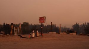
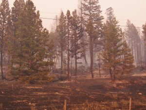
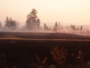
At about 8:00 pm we passed through Alexis Creek heading towards the fire. The winds were from the west blowing smoke away from us, so we had good views of the Hanceville fire on the hills to both the north and south of Highway 20. Fire crews and heavy equipment were working to put in fire guards to protect homes in the Anaham Reserve. As we drove further east, the fire came closer to the road and we drove through areas that had already been largely burned, with residual spot fires that were still active. Lee’s Corner gas station and restaurant was burned down. Proceeding further east from Lee’s corner, we drove into the active fire area, with burning on both sides of the road. This is where some of the video begins.

Visualize for a moment a massive fire that is many square kilometers in size working it’s way through a somewhat open conifer forest and grasslands that are tinder dry. A westerly wind is pushing a plume of smoke to the east. The plume is thin on the west edge and rises like a massive wedge as you move to the east. We were driving from the thin edge of the smoke wedge into the thick edge. It got steadily darker.

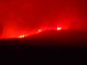
The fire was burning to the road edge on both sides and there was some crowning visible (for non-foresters, crowning is when the fire burns explosively through the foliage in the upper part of a tree). As it got darker the flames appeared more orange. Proceeding further east the darkness became complete and we forgot that the sun had not yet set. We saw periodic crowning, burning stems, and ground-level fires of varying intensity burning erratically on both sides of the road. Whole stands of trees in some spots had turned to red hot, glowing columns of orange light. Driving through the smoke was like driving through a blizzard. The road was only visible with the headlights on low beam and we could only see from 10 to 30 meters ahead. Several times intense fire-generated winds swept across and totally obscured visibility. Sparks and embers were common.

View video here: https://www.youtube.com/watch?v=860OpMy8kYc&t=2s

We proceed east through the dark with the fire on either side for about 20 km (from just after the old mill at the top of the Hanceville hill to about Harper Lake). At Harper lake the smoke began to clear somewhat and the fire was further from the road. It was still very dark, but we were able to use high beam and see further ahead. Ominous glows appeared here and there through the smoke and we were very concerned that we might drive into still more of the intense part of the fire. Finally a brighter orange glow appeared ahead and on both sides. Our first reaction was fear that the worst of the fire still lay in front of us. We were relieved, however, when we realized that this new glow was daylight and we were finally emerging from the fire.

Why didn’t we turn back early on? The trees in this area are not large (few over 20 m in height) and the sides of the road are cleared back some 20 or more meters. The chance of the road being blocked by a fallen tree was very small. We knew that the darkness was due to the thickening of the smoke wedge above us, and although the fire in the darkness looked frightening, it was in reality no worse than what you see in the early part of the video. We monitored the external temperature as we drove. It was about 22C as we entered the fire and increased to about 25 to 27 degrees. A couple of times it spiked to about 35 degrees and we considered turning around, but each time it quickly returned to the mid to high 20’s. As ominous as it all seemed, we were not in serious danger as long as we drove carefully and the outside temperature stayed reasonably low. So, we pushed forward and after what began to seem like an interminable amount of time, emerged on the east side of the fire. Our dog slept in the back, completely unaware of anything but the bag of treats in the glove box. Similar to a small group of cows we saw grazing in a small field, apparently oblivious to the fire all around them.

The video of a small part of our drive is here. Unfortunately, perhaps, Sally was so focused on the fire she lost focus on capturing more of it on video. Priorities.

There are many victims of this fire and the many other fires burning in central BC. This is the real issue. Please consider a donation to the Red Cross or another organization working to help people through this. In addition to our personal donations, we will also donate any funds we receive through commercial use of this video to the Red Cross relief effort.  https://donate.redcross.ca/ea-action/action?ea.client.id=1951&ea.campaign.id=74010&_ga=2.234106270.1847245054.1499898622-97910928.1499898622


03/7/17

CoAdapTree in pictures

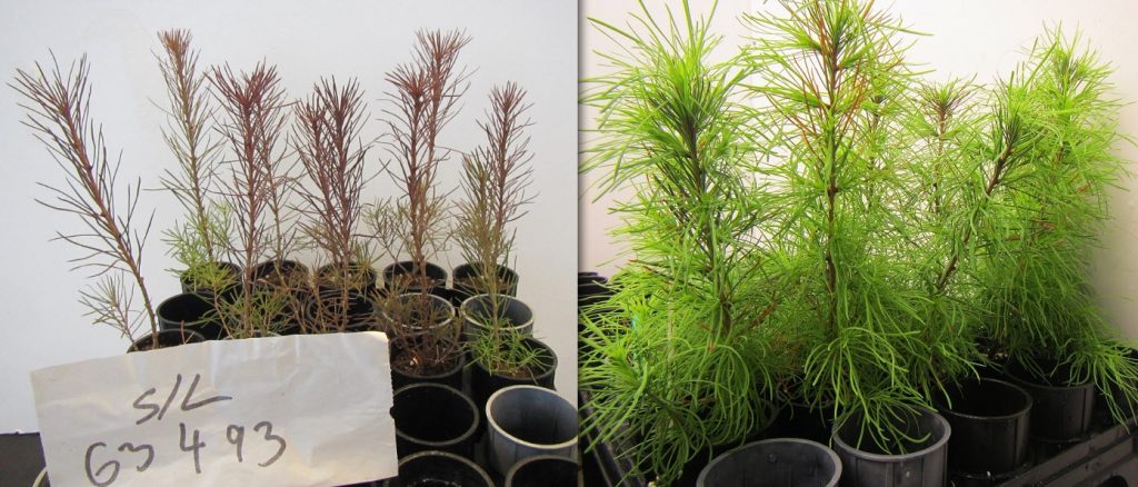
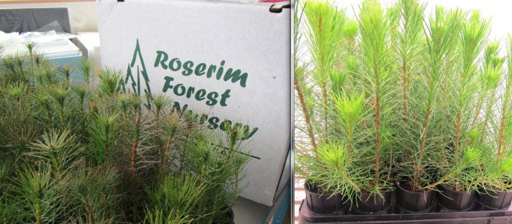
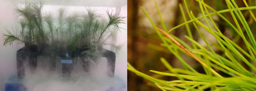
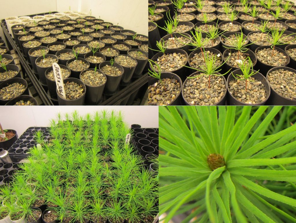
Here are some pictures showing the progress on our new project, CoAdapTree.

1. Western larch for transcriptome analysis


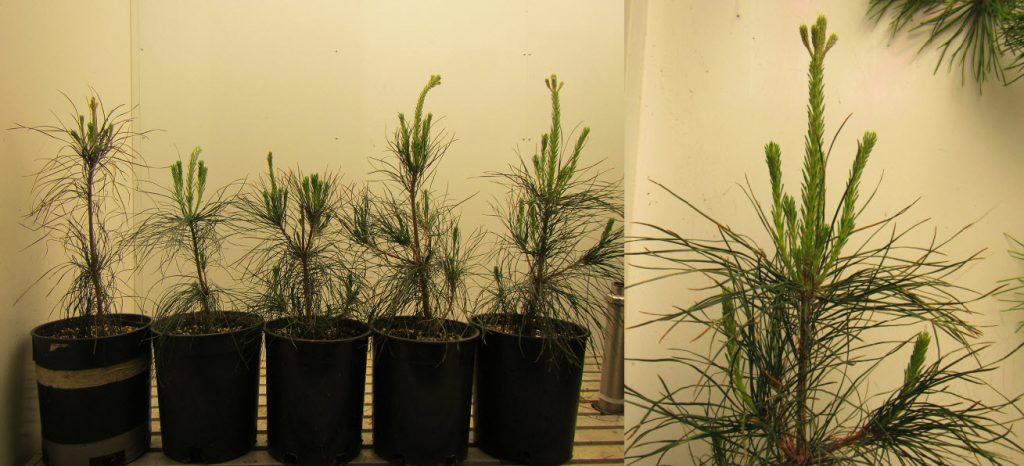
2. Lodgepole pine for inoculation pilot

3. Inoculation pilot

4. Lodgepole pine controlled crosses RxR and SxS

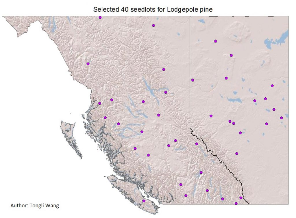
5. Pine : 40 seedlots

6. Collection of BC lodgepole pine (and some AB Jack pine): 40 seedlots

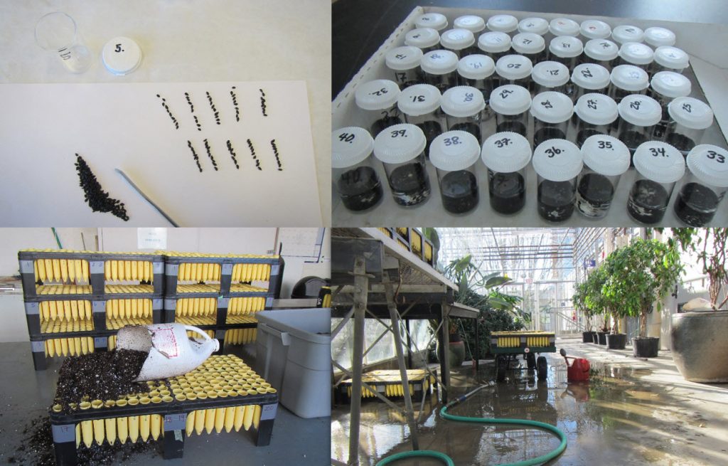
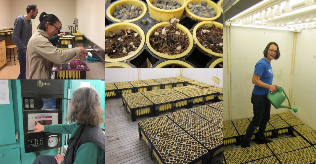
7. Sowing 4000 pine seedlings

8. Jack pine for transcriptome analysis


9. Jack pine RNA extraction


5.7