DID is a version of fixed effects estimation with panel data that can be used to estimate causal effects under the easily verifiable common trend assumption. A DID estimate captures the causal impact of a policy change by comparing the differences between the treated and control groups before and after the policy was implemented – the first difference is between before and after the policy intervention, and the second difference between the treatment and control groups. Now let’s look at two concrete examples where DID was used in Economics research.
Example 1: Gulati and Malhotra (2006)
On April 1, 1996, Canada and U.S. entered into a five-year contract called the Softwood Lumber Agreement (SLA henceforth), whereby a tariff rate quota was imposed on US-bound lumber exports from four Canadian provinces: Alberta, British Columbia, Ontario and Quebec. The first 14.7 billion board feet of softwood lumber from these provinces was exported duty free but further exports were subject to tariffs. A tariff of $50 per thousand board feet was imposed on the next 650 million board feet exported and further exports were going to be taxed at $100 per thousand board feet. The SLA was novel since exports from only four provinces were limited and other provinces were not subject to any restriction.
Gulati and Malhotra (2006) investigated firstly, whether the SLA caused a reduction in softwood exports to the U.S. from the four provinces and if so, what was the size of the decline. Secondly, what was the size of the increases, if any, in the softwood lumber exports of the other provinces to the U.S.
The regression equation they run is the following:
Xit = α0 + α1*Yit + α2*YUS,t + α3*Distt + α4*Ext + α5*RUS,t + α6*SLAi + α7*Restt + α8*SLAi*Restt + ut
and the STATA command will be:
reg X Yi YUS Dist Ex R SLA Rest SLA#Rest
where, Xit is log value of exports or log quantity of exports (annual) from province I to US. Yit and YUS,t are the log GDP of province i and US at time t respectively to control for demand of lumber in Canada and US. Disti is the log of distance from province I to the US border. RUS,t is the US interest rate to control for influence of interest rates on demand for new homes (a major source of softwood lumber). Ext is the US-Canada interest rate to control for price effects since exchange rates affect the relative price of Canadian lumber. SLA is a dummy variable which takes the value 1 for provinces on which tariffs were applied under SLA and 0 otherwise. Rest is a dummy for the years SLA was in effect and 0 otherwise. SLA*Rest is an interaction term that takes the value 1 for provinces under SLA for the years SLA was in place.
The key coefficient of interest is α8 as it is interpreted as the causal effect of the SLA on the change in exports of the SLA provinces compared to the non-SLA provinces. To understand why α8 is referred as the “Difference in Difference” estimate, take a look at the following table which is Table 4 in the paper.
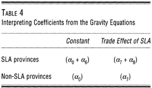
α6 captures the difference in the mean of log exports for SLA and non-SLA provinces before the SLA restrictions came into effect. α7 captures the effect of the SLA agreement on the non-SLA provinces. α7 + α8 reflects the effect of the SLA contract on the provinces named in the contract. Thus, α8 shows the difference in export performance of the provinces named in the SLA vs. not included in the SLA because of the SLA restriction.
Their results indicate that the SLA had a significant impact on the exports of non-SLA provinces and the SLA by itself increased the exports from these provinces compared to the SLA provinces by four times. But, the SLA lead to a decrease in exports of SLA provinces of only 5 percent which was statistically insignificant. Thus, SLA caused an increase in the exports of the non-SLA provinces rather than decrease in exports of SLA provinces.
Example 2: Card and Krueger (1994)
On April 1, 1992, New Jersey raised the state minimum wage from $4.25 to $5.05. However, right across the Delaware river, in Pennsylvania, minimum wages were kept unchanged at $4.25. Thus, if a researcher wanted to study the causal impact of minimum wage on employment, then comparing the difference in employment between New Jersey and Pennsylvania before and after April 1992 would be ideal for a DID. Card and Krueger (1994) did precisely that by studying the impact of the statutory minimum wage increase on employment at fast food restaurants where most minimum wage workers are employed. In practice, this is implemented in a simple panel regression with state and time fixed effects along with an interaction term:
Yist = α + µDt + φds + βDtds + uist ,
where Yist is the employment at restaurant i in state s at time t; Dt is a time-dummy variable, which takes the value 1 for periods after the minimum wage increase and takes the value 0 otherwise; and ds is a state-dummy variable, which takes the value 1 for the treated state (New Jersey) and 0 for the control state (Pennsylvania). The key coefficient of interest is β, the coefficient of the interaction between the state and time dummies, as it is interpreted as the causal effect of a minimum wage increase on employment. To understand why β is the so-called “Difference in Difference” estimate, a quick look at the following table of the conditional expectation of Yist will suffice:
| Before (Dt=0) | After (Dt=1) | Difference in Dt | |
| Pennsylvania (ds=0) | α | α+µ | µ |
| New Jersey (ds=1) | α+φ | α+µ+φ+β | µ+β |
| Difference in ds | φ | φ+β | Difference in Difference: β |
In short, DID estimate = (Difference in pre- and post-treatment outcomes for treated group) minus (Difference in pre- and post-treatment outcomes for control group).
Note that the panel regression set-up above can be reduced to a cross-sectional regression in first-differences by first averaging employment across all restaurants in a state, and then taking the difference between pre- and post-treatment periods.
ΔYs = µ* + βds + Δus
Here, ΔYs is the change in average employment is state s between the pre- and post-treatment periods, and ds is the same state-dummy variable as above. This reformulation of the panel regression in terms of a cross-sectional regression definitely reduces data requirements significantly.
One useful feature of implementing DID through regressions like above is that one is not limited to studying policy interventions that are binary in nature. For example, Card (1992) studies the impact of a federal minimum wage rise from $3.35 to $3.80 that has a differential impact across 51 U.S. states. Some U.S. states have minimum wages a little higher than the federal minimum, some a lot higher, and some are the same. The minimum wage is, therefore, a variable with different treatment intensity across states. In such a scenario, where the treatment intensity varies across different treatment groups, instead of using the dummy variable ds, one should use the pre-treatment level of intensity of the treatment, Xs. In the minimum wage study, Card (1992) uses the baseline (pre-increase) proportion of each state’s teenage labour force earning less than $3.80 as the measure of Xs. Card's specification was simply,
ΔYs = µ* + βXs + Δus .