Dummy variables or categorical variables arise quite often in real world data. For example, choosing between investing or not in a company’s share is a decision variable that can only take two values: YES or NO. Similarly, deciding which continent to spend your next vacation in can only take certain specific values: Asia, Africa, Europe, South America, etc. Categorical variables can not only capture situations where there is no inherent ordering of the options (like the above two examples, or say male versus female, etc.) but also when the values carry ordinal meaning (e.g., how happy are you at the moment on an integer scale of 1 to 5 with 5 being the happiest, or how democratic is a country’s politics on an integer scale of 1 to 10 with 10 being the perfect democracy).
A. Dummy Explanatory Variable: When one or more of the explanatory variables is a dummy variable but the dependent variable is not a dummy, the OLS framework is still valid. However, one should be cautious about how to include these dummy explanatory variables and what are the interpretations of the estimated regression coefficients for these dummies. First, one must be careful to include one less dummy variable than the total number of categories of the explanatory variable. For example, if the categorical variable ‘sex’ can take only 2 values, viz., male and female, then only one dummy variable for sex should be included in the regression to avoid the problem of muticollinearity. Including as many dummy variables as the number of categories along with the intercept term in a regression leads to the problem of the “Dummy Variable Trap”. So the rule is to either drop the intercept term and include a dummy for each category, or keep the intercept and exclude the dummy for any one category.
To provide an example, let us suppose our sample of individuals have five levels of wealth; poorest, poorer , middle , richer and richest. We are interested in understanding the relation between total number of children born in a family and their wealth level. (The data can be found here.)
We can create 5 dummy variables, called poorest, poorer , middle , richer and richest. The variable poorest takes the value 1 for individuals who have the poorest wealth and 0 otherwise. The variable poorer takes the value 1 for individuals who have poorer wealth and 0 otherwise. Similarly, we construct the other variables. We can take two approaches while regressing total number of children born in a family on wealth levels:
I. Include the constant term, poorest, poorer , middle , richer in the regression and drop richest.
The regression looks like
v201j = b0 + b1*poorestj + b2*poorerj + b3*middlej + b4*richerj +uj
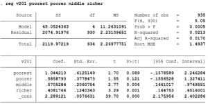
- The constant gives the expected number of children born in a household with the richest wealth level since v201j = b0 when all the variables take the value 0.
- The coefficient of poorest is interpreted as the difference between the expected number of children born in the household with the poorest wealth level and the richest wealth level. This is true because v201j = b0 + b1 when poorest=1 and all other variables are zero.
- Similarly, the coefficient of the other coefficients show the difference between the expected the number children born in the household with that particular wealth level and the richest wealth level.
II. Exclude the constant term, and include all the 5 variables.
The regression will look like:
v201j = b0*richestj + b1*poorestj + b2*poorerj + b3*middlej + b4*richerj +uj
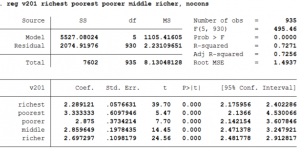
- Now in this regression, each coefficient gives the expected number of children born in the household given that particular wealth level. As you can see, the coefficient of richest is the same as the constant in the first method.
III. Include the constant term and all 5 variables.
Such a regression leads to multicollinearity and Stata solves this problem by dropping one of the dummy variables.
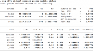
- Stata will automatically drop one of the dummy variables. In this case, it displays after the command that poorer is dropped because of multicollinearity.
- The constant term now reflects the expected number of children born in the poorer households. The coefficient is 2.875 which is the same as in the table before.
- The interpretation of the other coefficients is similar to the first example with the exception that now the base group is poorer household instead of richest as in the first example.
B. Dummy Dependent Variable: OLS regressions are not very informative when the dependent variable is categorical. To handle such situations, one needs to implement one of the following regression techniques depending on the exact nature of the categorical dependent variable.
Do keep in mind that the independent variables can be continuous or categorical while running any of the models below. There is no need for the independent variables to be binary just because the dependent variable is binary.
(i) Logistic Regression (Logit): A logistic regression fits a binary response (or dichotomous) model by maximum likelihood. It models the probability of a positive outcome given a set of regressors. When the dependent variable equals a non-zero and non-missing number (typically 1), it indicates a positive outcome, whereas a value of zero indicates a negative outcome. Mathematically speaking, running a logit of the dependent variable y on the regressors x1 and x2 basically fits the following model by estimating the coefficients b0, b1 and b2: Prob (yj = 1 | x1j, x2j) = exp(b0+b1x1j+b2x2j) / [exp(b0+b1x1j+b2x2j) + 1]. The specific functional form of the probability arises from the assumption of a logistic distribution for the error term in the regression.
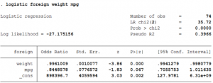
As an example, if we have data on weight and mileage of 22 foreign and 52 domestic automobiles, we may wish to fit a logit model explaining whether a car is foreign or not on the basis of its weight and mileage. (The data can be found here.)
The STATA command to run a logit model is as follows:
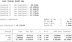
Here the dependent variable foreign takes the value 1 if the car is foreign and 0 if it is domestic. The regressors weight and mpg are usual continuous variables and denote the weight and mileage of the car respectively.
- The above STATA command yields estimates of the three coefficients: one constant/intercept, and the two coefficients for weight and mileage.
- The coefficient of weight implies that a unit increase in weight reduces the logs odds of the car being foreign (vs. domestic) by -0.004.
- The coefficient of mpg implies that a unit increase in mileage reduces the logs odds of the car being foreign by -0.17.
- The fourth column in the table shows the level of significance of the null hypothesis that the coefficient is equal to zero can be rejected. All the coefficients are statistically significantly from zero at the 10% level of significance.
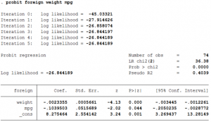
Sometimes, the researcher is not interested in the coefficients b0, b1 and b2 per se but in the odds ratios of the individual regressors, namely, exp(b0), exp(b1) and exp(b2).
This can be implemented in STATA using the following command:
- Now, the coefficient of weight implies that a unit increase in weight of the car increases the odds of the car being foreign by a factor of 0.996.
- The coefficient of mileage shows that a unit increase in the mileage of the car increases the odds of the car being foreign by 0.84.
One must be cautious when interpreting the odds ratio of the constant/intercept term. Usually, this odds ratio represents the baseline odds of the model when all predictor variables are set to zero. Howeer, one must verify that a zero value for all predictors actually makes sense before continuing with this interpretation. For example, a weight of zero for a car does not make sense in the above example, and so the odds ratio estimate for the intercept term here does not carry any meaning.
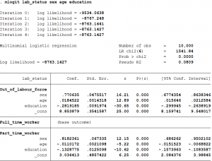
(ii) Probit Regression (Probit): One can change the distributional assumption of a logistic regression by assuming a standard normal distribution instead of the logistic distribution for the probability of a positive outcome. In other words, Prob.(yj = 1 | x1j, x2j) = φ(b0+b1x1j+b2x2j) where φ(.) denotes the cumulative distribution function of a standard normal distribution. This model is called a Probit model.
Let us return to our previous example and run a probit model rather than a logit model. This can be implemented in STATA using the following command:
- The regression coefficients have the same interpretation as the Logit model, i.e., the coefficient of weight implies that a unit increase in weight reduces the logs odds of the car being foreign (vs. domestic) by -0.004.
- As can be seen, all the coefficients are quite similar to the logit model.
- The choice of logit or probit model depends on economic theory and preference of the researcher.
Note: Both the Logit and Probit models are suitable when the dependent variable is binary or dichotomous. When the dependent variable has more than two categories, one needs to implement either a multinomial logistic regression or an ordered logistic regression, discussed below.
(iii) Multinomial Logit: In a multinomial logit model, the number of outcomes that the dependent variable can possibly accommodate is greater than two. This is the main difference of the multinomial from the ordinary logit. However, multinomial logit only allows for a dependent variable whose categories are not ordered in a genuine sense (for which case one needs to run an Ordered Logit regression).
Consider a regression of y on x where the categorical dependent variable y has 3 possible outcomes. In the multinomial logit model, one estimates a set of coefficients b0(1), b1(1), b0(2), b1(2), b0(3), b1(3), corresponding to each outcome:
Prob (y =1) = exp(b0(1) + b1(1)x) / [ exp(b0(1) + b1(1)x) + exp(b0(2) + b1(2)x) + exp(b0(3) + b1(3)x) ]
Prob (y =2) = exp(b0(2) + b1(2)x) / [ exp(b0(1) + b1(1)x) + exp(b0(2) + b1(2)x) + exp(b0(3) + b1(3)x) ]
Prob (y =3) = exp(b0(3) + b1(3)x) / [ exp(b0(1) + b1(1)x) + exp(b0(2) + b1(2)x) + exp(b0(3) + b1(3)x) ]
This model, however, is unidentified in the sense that there is more than one solution to b0(1), b1(1), b0(2), b1(2), b0(3), b1(3), that leads to the same probabilities for y=1, y=2 and y=3. To identify the model, one needs to set b0(k) = b1(k) =0 for any one of the outcomes k=1, 2 and 3. That outcome is called the base outcome, and the remaining coefficients will measure the change relative to that y=k group. The coefficients will differ because they have different interpretations, but the predicted probabilities for y=1, 2 and 3 will still be the same. For example, setting b0(2) = b1(2) =0, the equations become
Prob (y =1) = exp(b0(1) + b1(1)x) / [ 1 + exp(b0(1) + b1(1)x) + exp(b0(3) + b1(3)x) ]
Prob (y =2) = 1 / [ 1 + exp(b0(1) + b1(1)x) + exp(b0(3) + b1(3)x) ]
Prob (y =3) = exp(b0(3) + b1(3)x) / [ 1 + exp(b0(1) + b1(1)x) + exp(b0(3) + b1(3)x) ]
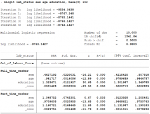
As an example, an individual’s choice of not being in the labour force, becoming a full-time worker or a part-time worker could be modeled using their education and control for age and sex. (The data can be found here.).
We have defined the variable lab_status as containing the employment and labour force participation of an individual. 0 refers to not in labour force, 1 refers to full-time work and 2 refers to part-time worker. The variable sex is defined as male taking the value 1 and female taking the value 2.
To implement such a multinomial logit in STATA, the following command can be run:
mlogit lab_status sex age education
- The coefficient of sex implies that the relative log odds of being out of the labor force vs. being a full-time worker will increase if the individual is a female vs. male.
- The coefficient of sex implies that the relative log odds of being a part-time worker vs. being a full-time worker will increase if the individual is a female vs. male.
- A one unit increase in age is associated with a 0.018 increase in the relative log odds of being out of the labor force vs. being full-time employed.
- A one unit increase in age is associated with a 0.011 decrease in the relative log odds of being part-time employed vs. being full-time employed.
- The coefficient of education implies a one year increase in years of schooling decreases the relative log odds of being out of the labor force vs. full-time employed by 0.28.
- The coefficient of education implies a one year increase in years of schooling is associated with a 0.13 decreases in the relative log odds of being part-time employed vs. being full-time employed.
The above command allows STATA to arbitarily choose which outcome to use as the base outcome. If one wants to specify the base outcome, it can be done by adding the base() option. Suppose, we want to compare with being out of the labor force rather than full-time worker. In this case the base outcome is 0 and to implement it in Stata we will run the following command:
mlogit lab_status sex age education, base(0)
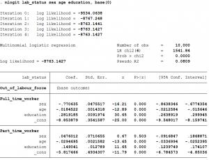
- This tells STATA to treat the zero category (y=0) as the base outcome, and suppress those coefficients and interpret all coefficients with out-of the labor force as the base group. The value in the base category depends on what values the y variable have taken in the data.
- The coefficient of sex, age, education and constant have flipped signs but have the same magnitude on those for a full-time employed individual compared to those for out-of the labor force in the previous case. This is to be expected as we have flipped the base group.
- The coefficient of sex implies that the relative log odds of being part-time employed vs. out of the labor force will only slightly increase if the individual is a female vs. male.
- A one unit increase in age is associated with a 0.029 decrease in the relative log odds of being part-time employed vs. out of the labor force.
- A unit increase in the years to schooling is associated with a 0.15 increase in the relative log odds of being part-time employed vs, out of the labor force.
Similar to odds-ratios in a binary-outcome logistic regression, one can tell STATA to report the relative risk ratios (RRRs) instead of the coefficient estimates. The relative risk ratio for a one-unit change in an explanatory variable is the exponentiated value of the correspending coefficient. So, for example when the base outcome is y=2, the relative risk of y=3 is the relative probability [Prob(y=3)/Prob(y=2)] = exp(b0(3) + b1(3)x). Then the relative risk ratio (RRR) of y=3 for a one-unit change in x is given by exp(b1(3)), which is what STATA reports when the rrr option is turned on.
This is done by the following command:
mlogit lab_status sex age education, base(0) rrr
- The relative risk ratio of an extra year of schooling is 1.16 (exp(0.15)) for being part-time employed vs. out of labor force.
(iv) Ordered Logit: In an ordered logit model the actual values taken on by the categorical dependent variable are irrelevant, except that larger values are assumed to correspond to ‘higher’ outcomes. Such dependent variables are often called ‘ordinal‘, for instance, ‘poor’, ‘good’, and ‘excellent’, which might indicate a person’s current health status or the repair record of a car.
In ordered logit, an underlying score is estimated as a linear function of the explanatory variables and a set of cutoffs. The probability of observing outcome k, Prob (y=k), corresponds to the probability that the estimated linear function, plus the random error, is within the range of the cutoffs estimated for the outcome: Prob (yj = k) = Prob ( ck-1 < b0 + b1x1j + b2x2j + uj < ck) where the error term uj is assumed to be logistically distributed. STATA reports the estimates of the coefficients b0, b1 and b2 together with the cutoff points c1, c2, … , cK-1, where K is the number of possible outcomes of y. c0 is taken as negative infinity, and cK is taken as positive infinity.
Let’s consider the following example: We want to model the choice of the total number of children born in a family using data on the daughter to son ratio (v203/v201), education (v133), age of the spouse (v012) and wealth quintile dummies. We can create 5 dummy variables, called poorest, poorer , middle , richer and richest. The variable poorest takes the value 1 for individuals who have the poorest wealth and 0 otherwise. The variable poorer takes the value 1 for individuals who have poorer wealth and 0 otherwise. Similarly, we construct the other variables. (The data can be found here.)
Ordered logits can be implemented in STATA using the following command:
ologit v201 daughter_son_ratio v133 v012 poorest poorer middle richer
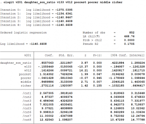
- A unit increase in the daughter to son ratio will increase the log odds of having another child by 0.86.
- A unit increase in the years to schooling (v133) will reduce the log odds of having another child by 0.16.
- The log odds of having another child increases as age increases.
- The omitted wealth quintile in the regression is the richest wealth quintile. Thus, the poorest household has a higher log odds of 1.51 of having a child compared to the richest household.
- Similarly, middle and richer households have a higher log odds of having another child compared to the richest household.
To, obtain the odds ratio instead of the log odds, we need to use the or option. To implement it in Stata, we need to run the following command:
ologit v201 daughter_son_ratio v133 v012 poorest poorer middle richer, or
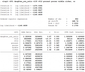
- A unit increase in the daughter to son ratio will increase the odds of having another child by 2.35.
A model with categorical dependent variable: Another Example
Consider the possible outcomes 1, 2, 3, …, k of the dependent variable y. Suppose k=3 — “buy an American car”, “buy a Japanese car”, and “buy a European car”. The values of y are then said to be ‘unordered’. Even though the outcomes are coded as 1, 2 and 3, the numerical values are arbitrary because 1<2<3 does not imply that outcome 1 (buy American) is less than outcome 2 (buy Japanese) is less than outcome 3 (buy European). This unordered categorical nature of the dependent variable distinguishes the use of mlogit from regress (which is appropriate for a continuous dependent variable), from ologit (which is appropriate for ordered categorical data), and from logit or logistic or probit (which are suitable for only k=2 or binary outcomes, which may or may not be thought of as ordered).
