Regression with Count Variable

When the dependent variable is a non-negative count variable, the standard OLS regression is no longer valid. Typically, the Poisson regression or some variation of it is used to analyze such count data. Here we will discuss the Poisson, Negative Binomial, and Zero-Inflated Negative Binomial regressions along with their STATA implementations.

Poisson Regression

Poisson regression fits models of the number of occurrences (counts) of an event where it is assumed that the number of occurrences follow a Poisson distribution. The Poisson distribution has been applied to diverse events with the following basic assumptions:

There is a quantity called the incidence rate that is the rate at which events occur, e.g., 5 per second, 20 per square metre, etc.
The incidence rate can be multiplied by exposure to obtain the expected number of observed events, e.g., a rate of 5 per second multiplied by 30 seconds means that 150 events are expected.
Over very small exposures, the probability of finding more than one event is small compared with the exposure length.
Non-overlapping exposures are mutually independent.

With these assumptions, to find the probability of k events in an exposure of size E, one divides E into n sub-intervals, and approximate the answer as the binomial probability of observing k successes in n trials. By letting n to be arbitrarily large, one obtains the Poisson distribution.

In the Poisson regression model, the incidence rate of the j^th observation is assumed to be given by r_j = exp(b₀+b₁x_1j+b₂x_2j) if x₁ and x₂ were the two explanatory variables. If E_j is the exposure, the expected number of events will be C_j = exp[ln(E_j)+ b₀+b₁x_1j+b₂x_2j].

The parameters are computed using a log-likelihood function which is:

lnL = ∑ [ y_j*β*x – r_j – lny_j!]

Example:

We have data on the number of deaths, average age in months and the total number of person-years of exposure to risk of the children between birth and age 10 for three cohorts of children born in 1941–49, 1960–67, and 1968–76. We want to understand how the deaths of the children changes with age of the children. This falls under running a regression with Count variable and a Poisson regression can be implemented (to install the data in Stata, type: webuse rod93, clear). Before we run a Poisson regression, generate logexposure as natural log of exposure.

poisson deaths age_mos, exposure(logexposure)

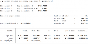
The option exposure() dictates STATA to restrict the coefficient of ln(logexposure) to be 1. Note that without the exposure() option, the exposure E_j is assumed to be 1.
The coefficient of age_mos implies that the expected change in the log count of the number of deaths as age increases by one unit is -0.017.

Often in Poisson regressions, one is interested in comparing the incidence rates. This is easily done by calculating incidence-rate ratios (IRR). The IRR for a one-unit change in x_i is exp(b_i) or in other words, the ratio of the expected number of events for a unit increase in the explanatory variable to the expected number of events. The option irr tells STATA to report the incidence-rate ratios exp(b₁) and exp(b₂) instead of the coefficients b₁ and b₂.

poisson deaths age_mos, exposure(E) irr

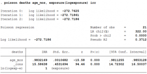
The table shows that the percent change in the number of deaths for a unit increase in age is (0.983-1) = -1.7%.

Negative Binomial (NB) Regression

Similar to a Poisson regression, in a Negative Binomial regression the dependent count variable is believed to be generated by a Poisson-like process, except that the variation is greater than that of a true Poisson. This extra variation is referred to as overdispersion, which may arise due to an omitted explanatory variable.

One derivation of the negative binomial mean-dispersion model is that individual units follow a Poisson regression model, but there is an omitted variable Z_j, such that exp(Z_j) follows a Gamma distribution with mean 1 and variance v: Y_j ~ Poisson(M_j) where M_j = exp(b₀ + b₁X_1j + b₂X_2j + ln(E_j) + Z_j) , exp(Z_j) ~ Gamma(1/v, v) and E_j is the exposure variable. We refer to v as the overdispersion parameter. The larger v is, the greater the overdispersion.

Example:

Lets, return to the above example. In STATA, a Negative Binomial (mean-dispersion) regression can be executed by the following command:

nbreg deaths age_mos, offset(logexposure)

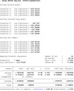
The option offset() is akin to the exposure() option in Poisson regression with the only difference being that offset() does not automatically transform the exposure variable into its natural logarithm. Nevertheless, offset() restricts the coefficient of e(=ln(E)) to be equal to 1 in the regression.
The coefficient of age_mos implies that the decrease in the expected log count of the number of deaths is 0.05.
STATA also reports the estimate of the overdispersion parameter v, which it calls alpha. It also reports the null hypothesis of alpha is equal to 0 in the last line of the output table. In a Poisson model, alpha is equal to 0 by assumption but in a Negative binomial model it is not. The test of the null hypothesis thus tells us if the Poisson model is appropriate or not. In this case, the null hypothesis that alpha is equal to 0 is rejected at lower than 1% level of significance, thus, the Poisson model is not the appropriate model to run.

STATA allows the overdispersion parameter to be modelled as a linear combination of some observable variables V₁ and V₂ (say), that is, ln(v_j) = c₀ + c₁V_1j + c₂V_2j.

Suppose, we think in our example that the overdispersion varies across cohorts. To implement such a specification in STATA, one needs to use the following command:

nbreg deaths age_mos, offset(logexposure) lnalpha(i.cohort)

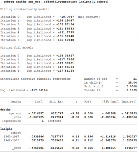
The command gnbreg stands for Generalized Negative Binomial Regression.
lnalpha() allows one to list the variables that affect the overdispersion parameter.
The interpretation of the coefficient on age remains the same as before.
Moreover, as we can see the coefficient on the lnalpha for the cohort 1960-1967 and 1968-1976 are slightly higher compared to the reference cohort 1940-1947, but these estimates are not significantly different so, overdispersion does not vary by cohorts.

In a mean-dispersion Negative Binomial regression, the dispersion for the j^th observation is equal to 1 + exp(b₀ + b₁X_1j + b₂X_2j + ln(E_j) ), that is, the dispersion for every observation is different. Another option is to have a constant dispersion, say (1+delta), across all observations. The constant-dispersion Negative Binomial regression model assumes M_j~ Gamma(exp(b₀ + b₁X_1j + b₂X_2j + ln(E_j))/delta, delta) instead of M_j~ Gamma(1/v, v.exp(b₀ + b₁X_1j + b₂X_2j + ln(E_j))) in the mean-dispersion model. The Poisson model corresponds to either d=0 or v=0 depending on the type of Negative Binomial model considered.

Continuing the example from Poisson regression, we can implement the Negative Binomial model in STATA with the following command:

nbreg deaths age_mos, offset(logexposure) dispersion(constant)

The output table is not shown for brevity.
The interpretation of the coefficient on age_mos remains the same as before.

How to choose between Poisson and Negative Binomial?

Step 1: Run the Poisson regression.

poisson deaths age_mos, exposure(logexposure)

Step 2: Run the goodness of fit test

estat gof

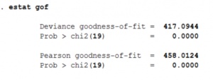
Step 3: If the Prob>chi2() is very close to zero (that is, lower than 0.05) then run the Negative Binomial regression. Else stick with the Poisson model. In this case, the p-value is very small so, the Poisson model is inappropriate for our example.

Zero-Inflated Negative Binomial (ZINB) Regression

Sometimes the count of zeros in a sample is much larger than the count of any other frequency. In other words, the number of zeros are inflated. In that case, instead of using the ordinary negative binomial or Poisson regression, one should run the Zero-Inflated Negative Binomial model. Obviously, how much zero-inflation is enough to call for the choice of this zer-inflated model is a matter of modelling preference, which is resolved by statistical tests discussed below. Specifically, one needs to test the ZINB model against both the ordinary NB model and the Zero-Inflated Poisson (ZIP) model.

A zero-inflated model assumes that zero outcome is due to two different processes. For example, if different groups of campers are asked how many fishes they caught, the response can be zero due to two separate reasons: one, a camper has gone fishing but did not catch a fish, and two, the camper did not go fishing at all. Thus the two processes here are that a camper has gone fishing versus not gone fishing (which is essentially a binary choice Logit model) and if gone for fishing then the count of the number of fish caught (which is the Poisson or Negative Binomial part of the count model). In other words, the expectation of the event that k fishes were caught is given by the formula, E(k fishes caught) = Prob(Not gone fishing)*0 + Prob(Gone fishing)*E(k fishes caught | Gone fishing).

Example:

Lets look at the following example, where we have data on 250 families that went to a park where they could do fishing if they wanted but we do not have data on whether a family fished or not. Each family was asked about how many fish they caught (count), whether or not they brought a camper to the park (camper), how many children were in the group (child), how many people (including children) were in the group (persons), and a dummy variable (livebait) which takes the value 1 if they brought a livebait while fishing and 0 otherwise.

We are interested in predicting the factors that affect the number of fish caught but also in predicting the number of excess zeros since our data has many of them (142 of 250). We will run the ZINB model in STATA along with the tests of model selection can be done using the following command:

zinb count child camper, inflate(persons) vuong zip nolog

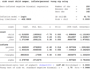
The coefficient of child implies that the expected change in log count for a one-unit increase in child is -1.51.
The coefficient of camper implies that a camper has a higher log count of fish caught (by .88) than a non-camper.
Both these results came from running a negative binomial model.
The option inflate() tells STATA that the variable person needs to be used to estimate the binary choice (or Logit) part of the process that generates the zero outcome.
The log odds of being an excessive zero would decrease by 1.67 for every additional person in the group.
The option vuong tests the zero-inflated negative binomial model with an ordinary negative binomial regression model. A significant z-test indicates that the zero-inflated model is preferred. The Vuong test suggests that the zero-inflated negative binomial model is a significant improvement over a standard negative binomial model.
The option zip tests the ZINB model against the ZIP model. A significant likelihood ratio test for the overdispersion parameter, alpha=0 indicates that the ZINB model is preferred to the ZIP model. We can see at the bottom of our model that the likelihood ratio test that alpha = 0 is significantly different from zero. This suggests that our data is overdispersed and that a zero-inflated negative binomial model is more appropriate than a zero-inflated Poisson model.