These are simple examples of useful commands and options using 1978 auto data from STATA. The commands are in bold text; variables and other inputs are in plain text for the sake of example.
Commands: SET UP
Do-Files
| doedit | Opens the Do-file editor. Here you can type a list of commands for your data analysis. The point of a Do-file is that you can reproduce the same results later, and you can revise it with more commands. |
| #delimit ; | (In Do-files only). Changes the line delimiter to a semicolon ";". All commands in the Do-file after this one must now end with a semicolon. This is helpful if you have a long command: you can split it into multiple lines in the do-file and mark the end of the entire command with a semi-colon. This makes for a cleaner output when the command is displayed in the results section upon execution. |
| #delimit cr | (In Do-files only). Resets the line delimiter to carriage return. All commands after this now end at the end of the line - a new line starts a new command. This is the default setting. |
| do "C:\documents\autoanalysis.do" | Executes all of the commands from the Do-file "autoanalysis" in order. If any command contains an error (syntax, misspelling, etc.), STATA will execute the commands up to that line only before stopping. In this case, reopen the editor and correct any mistakes. |
Log Files
| log using autoanalysis.log | Creates a file that records all of the results of your data analysis in a log. Specifying ".log" records your output as a text file, otherwise it is recorded as a STATA file ".smcl" that opens in the viewer. The log file will be stored in the folder under the current directory. |
| * comment on data analysis | Starting a command line with an asterisk "*" makes the command line act as simple text - it won't be interpreted as a command. This is helpful in do-files and log files as a way to leave notes on your analysis when you review the file later. |
| log off log on |
"log off " temporarily suspends the log file, and "log on" reopens it. This is helpful if you want to perform some data analysis without including the results in the log file, and if you want to reopen the log file later in the same session. |
| log close | Ends the log file. Any commands submitted and their results will no longer be stored in the log file. |
| log using autoanalysis.log, append | Reopens an existing log file. This lets you add more commands and results to the same log file. |
| translate autoanalysis.log autoanalysis.pdf | Reformats the log file "autoanalysis" from a text file to a pdf file. |
Importing Data
| cls |
Clears the results window. As an alternative to the command clear, cls keeps the data file in use |
| cd “C:\documents\data” | Changes the working directory to the specified folder. Input the folder which contains the data file we want to use. |
| use auto.dta, clear | Loads a data set from the current directory. The option clear clears the current dataset from memory. For all examples we use the auto data file included in STATA. |
| import excel “C:\documents\data\auto.xlsx”, sheet(“Sheet1”) firstrow | Imports the auto data if it were an excel file. sheet determines which worksheet to import, and firstrow imports the first row of the excel file as the variable names. |
| import delimited "auto.csv", rowrange(1:74) colrange(1:12) varnames(1) | Imports the auto data if it were a comma-separated values (.csv) file. Options rowrange and colrange specify ranges of rows (observations) and columns (variables) to import, respectively. varnames specifies which row contains the variable names - in this case, the first row. |
Exporting Data
| save auto.dta, replace | Saves the current data file and overwrites the old one. We can omit the replace command if we want to save the data under a new name. |
| export excel "autodata.xls", firstrow (variables) | Saves the current data file as a new excel file. The firstrow option uses the variable names as the first row of the excel file. Otherwise the variable names will be omitted. |
Commands: Data Management & Analysis
Summary Statistics
| describe mpg price | Displays the variable type, format and value labels for mpg and price. |
| count if foreign == 1 | Counts the number of observations that satisfy certain conditions. Here we count the number of foreign made cars. |
| summarize mpg price, detail | Displays summary statistics for variables mpg and price (mean, standard deviation, minimum and maximum). Option detail gives more statistics such as percentiles (50th percentile is the median), skewness, and kurtosis. |
| codebook mpg price | Displays variable type, summary statistics, percentiles, and number of missing values. |
| inspect mpg | Displays a simple histogram for mpg. Also gives the numbers of observations with negative, zero, or positive values; unique values; and missing values. |
| histogram mpg, bin(10) | Displays a histogram of mpg with parameters decided by STATA. Option bin(10) specifies number of bins. Width of each bin determined automatically by bin size and range of mpg. |
| browse make mpg price | Opens a data browser for variables make, mpg, and price. Helpful if you have many variables and want to focus on a subset of them. |
| tabulate rep78, missing | Displays a one-way frequency table. Option mi treats missing values as a separate category (otherwise observations withI missing values are ignored). Tabulate works best for discrete variables, or variables with few unique values. |
| tabulate mpg foreign | Displays a two-way frequency table. For each value of the first variable mpg, we tabulate the frequency for each value of foreign. It is important to list the variable with more unique values (mpg) first. |
| tabstat price weight mpg, by (foreign) stat (mean sd n) | Displays a table of summary statistics of price, weight, and mpg. Option by(...) generates separate statistics for each value of foreign. Option stat(...) determines which summary statistics to display (mean, standard deviation, and number of observations). |
| list make price mpg if mpg >= 30 | Lists the values of make, price and mpg for observations that satisfy the conditions determined by option if. In this case we list the values only for cars with mpg greater than or equal to 30. |
| correlate mpg weight price | Displays a correlation matrix for all specified variables. |
Generating Variables
| generate lprice = log(price) | Creates a new variable based on a function of existing variables. Here we take the (natural) logarithm of the variable price. The new variable lprice represents the log of price of every observation. This is a critical tool for model specification. |
| generate efficient = 1 if mpg >= 22 replace efficient = 0 if mpg < 22 |
Creates a dummy variable that takes on value 1 if the observation has above average gas mileage, and value 0 otherwise. The replace command fills in the missing values that are necessarily generated by the first command. Generally, replace is used to modify contents of an existing variable. |
Modifying Data
| rename headroom hdrm | Renames an existing variable. We can rename the variable headroom to hdrm for short. |
| drop headroom trunk length | Removes the variables headroom, trunk, and length from the data file. Note that drop (and keep) is irreversible. To retrieve these variables you have to clear and reopen the original data file. (Make sure you always have a copy of the original when you save data files.) |
| keep make price mpg rep78 foreign | Removes all other variables from the data file, and keeps only the specified variables. Most drop commands can be replaced with keep for this opposite effect. |
| drop if foreign == 1 | Drops all observations that satisfy the specified conditions. Here we want to look only at domestically produced cars, so we drop all observations where the foreign variable takes on value 1. |
| gsort -price keep in 1/20 |
Sorts the observations in a specified order of a variable, and then keeps the observations in a specified range. First we use gsort to arrange the observations in descending (-) order of price. Then we keep observations 1 to 20, dropping everything else. The resulting data set represents the observations of the top 20 most expensive cars. |
| keep if inrange(mpg,20,30) | Keeps the observations where the value of a variable lies within a specified range. Here we keep the cars with mpg between 20 and 30 (inclusive). |
| replace price = 4000 if price < 4000 | Replaces values of observations that satisfy certain conditions. Here we replace values of price lower than $4,000 with 4000. |
| recode mpg (12/22=0 "Inefficient")(23/41=1 "Efficient"), generate (Efficiency) | Recodes and generates a new dummy variable for mpg. We replace values from 12 to 22 with the value 0 and the label "Inefficient," and follow suit with values from 23 to 41. The generate option here creates a new recoded variable, otherwise the default is to replace the variable mpg. |
| mvdecode _all, mv(9999) | Decodes datasets that input the value "9999" for missing values. Here we replace all values of 9999 across all observations and variables with a missing value marker ".". |
| mvencode rep78, mv(9999) | Encodes missing variables in the current dataset to a specified value. Here we replace the missing values (denoted by ".") in the variable rep78 with a value of 9999. This is useful for exporting data. |
Commands: Regression Analysis
OLS Linear Regression
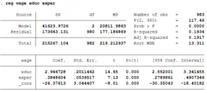
| regress price mpg foreign rep78 | Regresses independent variable price on dependent variables mpg, foreign and rep78 using ordinary least squares linear regression. Generates coefficients, standard errors, p-values , ANOVA table etc. |
| regress price mpg foreign rep78, robust | Option robust gives the robust standard errors and t-statistics. Generally robust is used to adjust for heteroskedasticity, and is usually justifiable with large sample sizes. |
| regress price mpg foreign rep78, noconstant | Option noconstant is used when the theoretical model calls for the intercept term to be zero. |
 |
Interpreting results |
Storing Values (After Regression)
| sca beta1 = _b[mpg] sca se1 = _se[mpg] sca obs = 74 |
Stores the values for later use. _b[mpg] denotes the beta coefficient from the last performed regression - and likewise with the standard error _se[mpg]. We can also store numbers such as the number of observations. This tool can be useful for manually calculating test statistics or for keeping track of values after running several regression models. |
| di beta1 di e(r2) |
Displays values in the results window - the capabilities are similar to that of sca. Here we display the value "beta1" which we previously stored, as well as the R-squared of the last performed regression. |
| gen beta1 = _b[mpg] label variable beta 1 "first specification mpg" |
Stores the beta coefficient for mpg as a variable with the label "first specification mpg." This is an alternative to sca if you need the value for later use if you are testing several model specifications - you can keep track of it in the variable list and give it a fitting label. |
| predict yhat |
Generates a new variable variable yhat based on the predicted values for each observation. |
Regression Diagnostics
Multicollinearity |
|
| pwcorr mpg foreign rep78, sig | Displays pairwise correlations between specified variables. Option sig displays significance levels for correlations. This is helpful in checking for multicollinearity. |
| vif | Displays the variance inflation factor for each independent variable. A VIF value greater than 10 suggests multicollinearity. |
Normality of Residuals |
|
| predict r, residual | Generates a new variable r based on the residuals of each observation from the linear regression. (See next command) |
| kdensity r, normal | Displays a kernel density estimate graph of the variable r. Option normal plots this graph against the normal distribution. Normality of the residuals is important for hypothesis testing |
| gladder price | Displays several graphs representing different transformations of the variable price. Each graph contains a histogram and a kernel density estimate. Normality of variables through choosing the proper functional form can help achieve normality of residuals. |
Homoskedasticity |
|
| rvfplot, yline(0) | Plots the residuals against the fitted values from the regression. Ideally, for homoskedasticity there should be no discernible pattern in the residuals' variance from the baseline y = 0. |
| estat hettest | Tests the hypothesis that the errors are homoskedastic. A high chi-squared statistic and a low p-value implies that the errors are heteroskedastic. |
Linearity |
|
| scatter r mpg | Displays a two-way scatterplot of the residuals against mpg. (see predict to generate residual "r"). Plot the residuals against each independent variable and check for non-linear relationships. |
| acprplot mpg, lowess | Displays an augmented component-plus-residual plot and a lowess smooth of the plotted points. It shows a scatterplot of all the points, a linear regression line, and a non-linear "lowess" curve. The relationship is linear if the lowess curve closely follows the linear regression line. |
Omitted Variable Bias |
|
| estat ovtest | Tests for omitted variable bias. A high F-statistic and a low p-value implies there may be omitted variable(s). |
Regression with Independent Variable being Dummy
Logit Regression |
|
| logit foreign weight mpg | A logistic regression fits a binary response model given a set of regressors to estimate the probability of a positive outcome. The specific functional form arises from the assumption of a logistic distribution for the error term in the regression. Displays the logs of odds ratios of the regressors. |
| logistic foreign weight mpg | Displays the odds ratios of the individual regressors. |
Probit Regression |
|
| probit foreign weight mpg | A probit regression fits a binary response model by assuming a standard normal distribution instead of the logistic distribution for the probability of a positive outcome. |
| Interpreting results for probit | |
Multinomial Logit Regression |
|
| mlogit lab_status sex age education | In a multinomial logit model, the number of outcomes that the dependent variable can possibly accommodate is greater than two and whose categories are not ordered in a genuine sense. This is the main difference of the multinomial from the ordinary logit. Displays coefficient of regressors with a randomly chosen base outcome. |
| mlogit lab_status sex age education, base(0) | The above command allows STATA to arbitarily choose which outcome to use as the base outcome. If one wants to specify the base outcome, it can be done by adding the base() option. |
| mlogit lab_status sex age education, rrr | Similar to odds-ratios in a binary-outcome logistic regression, one can tell STATA to report the relative risk ratios (RRRs) instead of the coefficient estimates, it can be done by adding the rrr option. |
| Interpreting results for mlogit | |
Ordered Logit Regression |
|
| ologit v201 daughter_son_ratio v133 v012 poorest poorer middle richer | In an ordered logit model the actual values taken on by the categorical dependent variable are irrelevant, except that larger values are assumed to correspond to ‘higher’ outcomes. Displays log odds of regressors. |
| ologit v201 daughter_son_ratio v133 v012 poorest poorer middle richer, or | To, obtain the odds ratio instead of the log odds, we need to use the or option. |
| Interpreting results for ologit |
Regression with Count variable
Poisson Regression |
|
| poisson y x, exposure( e ) | Poisson regression fits models of the number of occurrences (counts) of an event where it is assumed that the number of occurrences follow a Poisson distribution. y is the dependent variable, x is the independent variable and e is exposure or the expected number of observed events. |
| poisson y x, exposure( e ) irr | This option irr tells STATA to report the incidence-rate ratios. |
| estat gof | Test whether the Poisson regression or Negative binomial model is appropriate. |
| Interpreting results for poisson |
Negative Binomial Regression |
|
| nbreg y x, offset( e ) | In a Negative Binomial regression the dependent count variable is believed to be generated by a Poisson-like process, except that the variation is greater than that of a true Poisson. y is the dependent variable, x is the independent variable and e is exposure or the expected number of observed events. |
| nbreg y x, offset( e ) lnalpha( z) | This option tells STATA to model the overdispersion parameter as a linear combination of the observable variable z. |
| nbreg y x, offset( e ) dispersion(constant) | This option tells STATA to have a constant dispersion across all observations. |
| Interpreting results for nbreg |
Zero Negative Binomial Regression |
|
| zinb y x, inflate( z ) vuong zip | In a Zero Negative Binomial regression the dependent count variable the count of zeros is much larger than the count of any other frequency. y is the dependent variable, x is the independent variable and z is used as a regressor to explain the reason for such excess or inflated zeros. |
| Interpreting results for zinb |
Instrumental Variable Regression
| ivregress 2sls y x1 (x2 = z1) | Stata executes a two-stage least square where y is the dependent variable, x1 is an exogenous explanatory variable, x2 is the endogenous explanatory variable which is being instrumented by the variables z1. |
| Examples and more explanation |
Difference-in-Difference Regression
| reg y treatment time treatment#time | y is the dependent variable, treatment is a dummy variable with value 1 for treated group and 0 for control group, time is a dummy variable with value 1 when treatment started and 0 before treatment and the interaction between time and treatment captures the difference in difference coefficient. |
| Examples and more explanation |
Commands: Displaying Regression Results
Generating Regression Table
| ssc install estout | Installs a program that generates regression tables, see following commands for use. |
| eststo spec1 | Stores the last performed regression as one of the model specifications - spec1 - to be displayed in the table |
| esttab using AutoRegTable.smcl, se title (1978 Auto Analysis) | Exports a regression table with title "1978 Auto Analysis" comprised of all specifications previously stored with eststo command to the Stata file "AutoRegTable.smcl". Displays beta coefficients, standard errors (through option se), and significance stars. |
| translate AutoRegTable.smcl AutoRegTable.pdf | Converts the auto analysis regression table from a Stata file to a PDF file. |
Common Graphs
| histogram mpg, bin(10) |
Displays a histogram of mpg with parameters decided by STATA. Option bin(10) specifies number of bins. Width of each bin determined automatically by bin size and range of mpg. |
| scatter price mpg || lfit price mpg |
Displays a two-way scatterplot of variables price and mpg. "||" Allows us to overlay another graph on top - in this case, we overlay a line of best fit using option lfit. |
| graph matrix weight length mpg, half |
Displays scatterplots of every pairwise combination of variables. Option half omits the same graphs with reversed order. |
| kdensity price, normal | Displays a kernel density estimate of the variable price - a smoothed histogram essentially. Option normal plots the graph against the normal distribution for comparison. |
| graph bar price, over(rep78) | Displays a bar graph of the mean values for price for each value of rep78. This is helpful when the independent variable is continuous and the dependent variable is categorical. |
| graph hbox mpg, by(foreign) | Displays a box and whisker plot of the variable mpg. This represents the five number summary of the variable as well as outside values. Option by(foreign) generates two separate graphs representing mpg for foreign cars and for domestic cars. |
| gladder price | Displays several graphs representing different transformations of the variable price. Each graph contains a histogram and a kernel density estimate. |
| correlate mpg weight price | Displays a correlation matrix for all specified variables. |
| graph export PriceMpgScatter.pdf | Exports the graph currently displayed in the graph window as a PDF file titled "PriceMpgScatter". |
NOTE: This is not an exhaustive list of each command’s potential. For more options in STATA type “help” followed by the name of the command. You can also type “search” followed by a statistical term to find the exact command for that operation. You can replicate and explore these commands further by navigating the appropriate menus in the taskbar.
