OLS is a technique of estimating linear relations between a dependent variable on one hand, and a set of explanatory variables on the other. For example, you might be interested in estimating how workers’ wages (W) depends on the job experience (X), age (A) and education level (E) of the worker. Then you can run an OLS regression as follows:
Wi = b0 + b1Xi + b2Ai + b3Ei + ui.
Note that linearity of the regression model in OLS depends on the linearity of the parameters and not the linearity of the explanatory variables.
Non-Linearity of the Explanatory Variables
Non-Linearity of the Explanatory Variables
- In case age affects wages non-linearly (e.g., wage increases at a decreasing rate with age). This can be accommodated in the OLS framework by simply adding a quadratic term in age, like b4Ai2.
- Interaction between two or more explanatory variables can also be accommodated in OLS. For example, if one believes age and experience has a joint effect on wages then one can include the term b5AiEi.
- Another popular example where the explained and explanatory variables are non-linearly related but the explained variable is linear in the parameters, is a Cobb-Douglas production function, Y=AKαLβ. By taking logarithms on both sides of the production function, one can write,
ln(Y) = ln(A) + αln(K) + βln(L).
Thus an OLS regression can be run to estimate the production function parameters A, α and β as follows: ln(Yi) = b0 + b1ln(Ki) + b2ln(Li) + ui, where A=exp(b0), α=b1 and β=b2. Thus, linearity in parameters includes quite a large set of functional relations between the dependent and explanatory variables that can be estimated through OLS.The subscript i denotes the value of the corresponding variable for the ith worker in the dataset. If there are N workers, the subscript i runs from 1 through N. The parameters to be estimated are b0, b1, b2 and b3. Each of these parameters capture how the corresponding explanatory variable is related to workers’ wages w. For example, b2 captures how wages change, ceteris paribus, for one year increase in the worker’s age.
There are important variations and special cases of OLS that we will discuss in different contexts, e.g., panel regression, instrumental variable regression, regression discontinuity, difference-in-difference, etc.
STATA Command: See here
Suppose we are interested in understanding the effect of education of a person and experience on the job on wages of that person. To do so, we will regress wage on the two explanatory variables; educ (education) and exper (experience). (The data can be found here. )
This can be easily done in STATA using the following command:
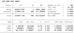
reg wage educ exper
- Alternatively one can type regress too instead of reg.
- STATA then estimates 3 parameters: the intercept term, the coefficient of educ and the coefficient of exper.
- The coefficient of educ means that for one year increase in schooling wages of that person will increase by $2.95.
- The coefficient of exper implies that for every extra year spent on the job increases the person’s wages by $0.38.
- The constant shows the average wage of a person with no schooling and no experience on the job. The value of the constant is -$24.38 which does not make sense since in our data the minimum years of schooling is 8. Thus, one needs to be careful while interpreting the constant since depending on the regression, the constant might or might not have a useful interpretation.
- The fourth and fifth column show the t-statistic and p-value of the null hypothesis that the coefficient is equal to zero. For all the coefficients we can reject that hypothesis since the p-value is less than 1%.
- The 95% Confidence interval implies that there is a 95% probability that the interval will contain the population parameter.
- The probability (Prob > F) tests whether the independent variables have no power to explain the dependent variables or not. Given a p-value of 0.000% we can reject the null hypothesis. In other words, the null hypothesis is that joint test whether all the coefficients are equal to zero or not. We can reject such a hypothesis and conclude that jointly the coefficients are significantly different from zero and they can predict the dependent variable.
- R2 is the percentage of the variance of the dependent variable to the variance of the independent variable. Thus, how much of the variation in the dependent variable that can be explained by the independent variables.
- Adjusted R2 compensates for the number of variables in the model. Adding another variable to the model will increase the Adjusted R2 only when the new variable improves the model fit more than expected by chance alone. Thus, Adjusted R2 will be less than R2 and it can be negative too unlike R2.
While estimating the parameters, it is customary to adjust the standard errors of the parameter estimates for heteroskedasticity. This is done by writing the following command:
reg wage educ exper, r
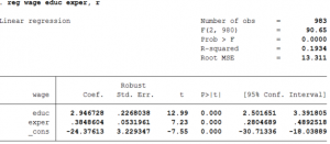
- Alternatively one can type robust instead of r after the comma.
- Note that the option ‘robust’ in STATA, only changes the standard error of the parameter estimates but not the estimates themselves.
- In this example, correcting for heteroskedasticity increased the standard error of education but reduced the standard error of experience.
Sometimes the theoretical model dictates that the intercept term is zero. Suppose we want to understand the relationship between the weight and length of a car. When the length of a car is zero then its weight should also be zero.
To run a regression of weight on length of the car with the additional impose restriction in STATA, one needs to write the following command (data can be found by typing: webuse auto, clear ) :
reg weight length, noconstant
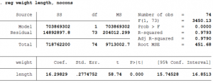
- In this case, STATA then estimates only 1 parameter: the coefficient of length.
