When the same cross-section of individuals is observed across multiple periods of time, the resulting dataset is called a panel dataset. For example, a dataset of annual GDP of 51 U.S. states from 1947 to 2018 is a panel data on the variable gdpit where i=1,…,51 and t=1,…,72.
The key difference in running regressions with panel data (with both cross-sectional and time-series variations) from a usual OLS regression (with only cross-sectional variation) is that one needs to control for the common effect for all individuals in a particular time point, and also the idiosyncratic individual effect that is common across all years. These are called the time fixed effects and the individual fixed effects respectively. The variation that is left after controlling for these fixed effects is the variation at the interaction between individual and time. The most common specification for a panel regression is as follows:
yit = b0 + b1xit + b2Di + b3Dt + eit
In the above regression, b2 denotes the individual fixed effects, while b3 denotes the time fixed effects. These fixed effects are nothing but the coefficients of the dummy variables Di and Dt. Once again, the problem of the dummy variable trap becomes relevant, as discussed in the section on regression with dummy variables. If there are N individuals, then only N-1 individual dummies (Di ‘s) should be included, and if there are T time-points, then only T-1 time dummies (Dt ‘s) should be included in the panel regression that contains the intercept term b0. The individual dummies are defined as follows: Di takes the value 1 if the data-point corresponds to individual i, and otherwise takes the value 0. Thus, Di will be 1 for T data-points and 0 for (N-1)T data-points. Similarly for the time dummies, Dt takes the value 1 if the data-point correponds to time-point t, and otherwise takes the value 0. Thus Dt will be 1 for N data-points and 0 for (T-1)N data-points.
Depending on whether the individual effects Di are allowed to be correlated with the explanatory variable xit , the regression model is either called a fixed effects (FE) model or a random effects (RE) model. While the uncorrelatedness of xit is desirable for both the FE and RE models, the RE model additionally imposes the independence of the individual effects Di with the explanatory variable xit . As a rule of thumb, it is always better to assume a fixed effects model because the estimates from an FE model is always consistent, while the RE model is consistent only if the underlying true model is RE. The only disadvantage of wrongly assuming an FE model when the true model is RE, is that the FE estimator will be inefficient (that is, the variance of the estimators will be larger). The Durbin-Wu-Hausman specification test helps the researcher to decide which model (RE or FE) to consider given a particular dataset.
Depending on the nature of the dependent variable yit, e.g., categorical type (binary or polytomous), or the endogeneity of xit, the techniques that have been discussed in different sections using cross-sectional data, are still largely valid with panel data.
STATA code without Example
In STATA, before one can run a panel regression, one needs to first declare that the dataset is a panel dataset. This is done by the following command:
xtset id time
The command xtset is used to declare the panel structure with 'id' being the cross-sectional identifying variable (e.g., the variable that identifies the 51 U.S. states as 1,2,...,51), and 'time' being the time-series identifying variable (e.g., the variable that records the year of observation 1947,1948,...,2018).
A fixed effects (FE) panel regression can be implemented in STATA using the following command:
regress y i.time i.id x
The i.time variable tells STATA to create a dummy for each time-point and estimate the corresponding time fixed effects. Similarly, i.id variable tells STATA to create a dummy for each individual and estimate the corresponding individual fixed effects. Another way to implement the FE model in STATA is to simply write the following command:
xtreg y i.time x, fe
The option fe tells STATA to include the cross-sectional effects and estimate them assuming an FE model. It should be noted that this alternative way of estimating the fixed effects model suppresses the estimates of the individual fixed effects. Therefore, if it is important to the researcher to know the estimates of the individual fixed effects then the first method is preferrable. On the other hand, if an RE model is to be fit, then it can be done in STATA using the following command:
xtreg y i.time x, re
STATA can also run the Durbin-Wu-Hausman specification test to help choose between the FE and RE models. The null hypothesis in the Hausman test is that the true model is RE against the alternative hypothesis that the true model is FE. Thus if the calculated test-statistic is large enough, or equivalently the p-value is small enough, then the FE model is preferred.
To do this, one first needs to estimate and store the estimates from each of the FE and RE models, and then compute the Hausman test-statistic to run the test. This is done as shown below.
xtset id time
xtreg y x, fe
estimates store fixed
xtreg y x, re
estimates store random
hausman fixed random
STATA code and Interpretation of output with Example
Suppose, we are interested in understanding the effect of financial development on GDP volatility. One might think that financial development might help households and firms to better manage unexpected events which will reduce the volatility in GDP. To perform such an analysis, we will need panel data on countries across time since countries differ in their levels of financial development and the rate of financial development (The data can be found here. Denzier et. al. (2002) is the seminal paper in this literature.).
The dataset also includes other macroeconomic variables such as degree of trade openness and GDP per capita. One might need to control for GDP since low income countries are expected to display higher volatility in output. Also, countries which are more open to trade might be more or less susceptible to foreign or domestic shocks. Obviously, this is not an exhaustive set of controls and more relevant controls can be added.
First we will declare the dataset is panel.
xtset ID time
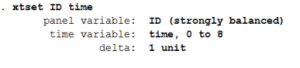
- Stata displays that the panel variable (ID) is strongly balanced implying that most countries are available with equal number of time periods otherwise it will show unbalanced. The analysis can be performed with unbalanced panel as well but having a balanced panel allows to better estimate the fixed effects.
- The time variable ranges from values 0 to 8. Depending on your dataset and application, you might require formating the time variable. (How to format time variable in Stata?)
- Delta shows the difference in the time units is 1.
Second, we will run the fixed effects model to investigate the relationship between financial development, given by ratio of total deposits in bank to GDP (deposits_gdp) and fluctuations in output given by standard deviation of filtered output (sd_gdp). There are controls for trade openness (tradeopenness) and log of per capita income (log_gdp_pc). The command to do this in Stata is the following:
xtreg sd_gdp deposits_gdp tradeopenness log_gdp_pc, fe
estimates store fixed
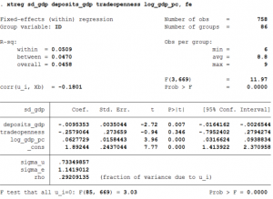
- The coefficient of deposits_gdp is -0.009 and it implies that a unit increase in finance reduces the standard deviation of GDP by 0.009. The coefficient is significantly different from zero.
- The important thing to keep in mind here, is that the coefficient reflects the effect from the time-variation. The fixed effects model controls for the individual effects so, only changes in the independent variable across time are captured and not differences in the independent variable between countries.
- The R2 within is the ordinary R2 (R2 in the cross-section OLS) in this case.
- sigma_u is the standard deviation of residuals within groups
- sigma_e is the standard deviation of the residuals of the idiosyncratic error term
- rho is the ratio of (sigma_u)2 / ( (sigma_u)2 + (sigma_e)2 ). It represents the intraclass correlation of the error. Thus, it explains the within country relative contribution.
- estimates will store the coefficients from the xtreg regression. We store it as fixed.
Third, we will now estimate this link using a random effects model. The command to do this in Stata is the following:
xtreg sd_gdp deposits_gdp tradeopenness log_gdp_pc, re
estimates store random
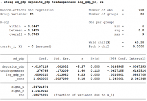
- The coefficient of deposits_gdp is -0.107 and it implies that a unit increase in finance reduces the standard deviation of GDP by 0.107. The coefficient is significantly different from zero.
- But the interpretation of the coefficient is different since it now measures the average effect of the independent variable on the dependent variable where the independent variables changes across time and countries by one unit.
- Since the random effects model is a weighted average of the between and within estimators, none of the three reported R2 are meaningful.
- The interpretation of sigma_u, sigma_e and rho is same as before.
- We store the coefficients as random.
To decide between fixed or random effects we can run a Hausman test where the null hypothesis is that the preferred model is random effects vs. the alternative that the preferred model is fixed effects.
hausman fixed random
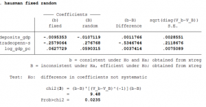
- The important thing to look at is the p-value of the test statistic and it is 2%. Thus, the Random effects model can be rejected.
