In Lab 2, we used the Fragstats software to analyse land use change around Edmonton between 1966 and 1976. The below maps show the land use maps in the entire study areas for each of the two years, using land use data downloaded from Canada Land Use Monitoring Program (CLUMP) data for Edmonton from the Geogratis website:

1966 Land Use in Edmonton
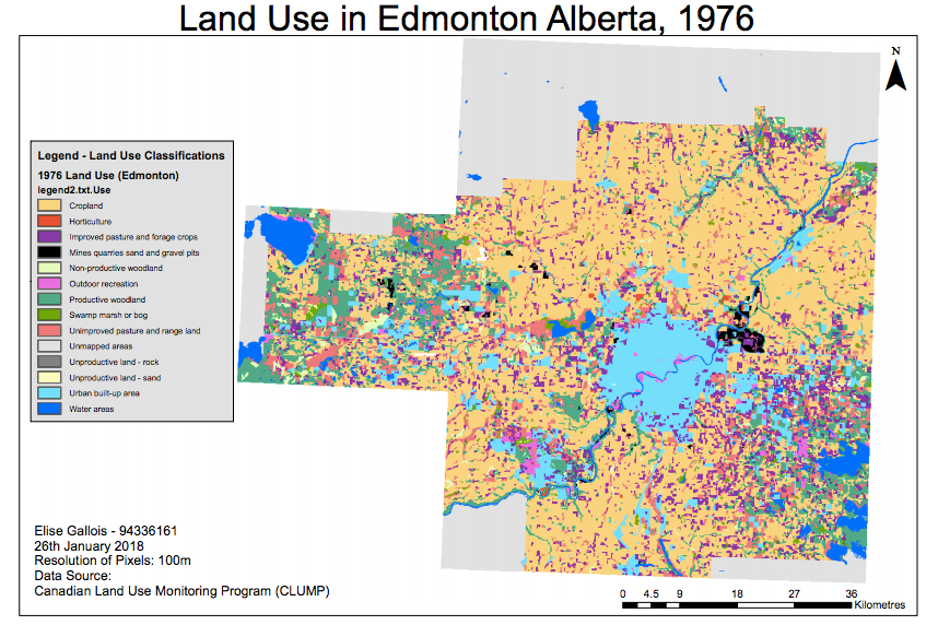
1976 Land Use in Edmonton
The Fragstats analysis revealed a number of noteworthy changes. One major trend is the decrease in cropland extent as land within this decade was converted to urban land, unimproved pasture, productive forest and mining. Urban areas increased in extent over this decade – both in the city of Edmonton and in smaller settlements, mostly located along the North Saskatchewan river, as can be seen in the map below:
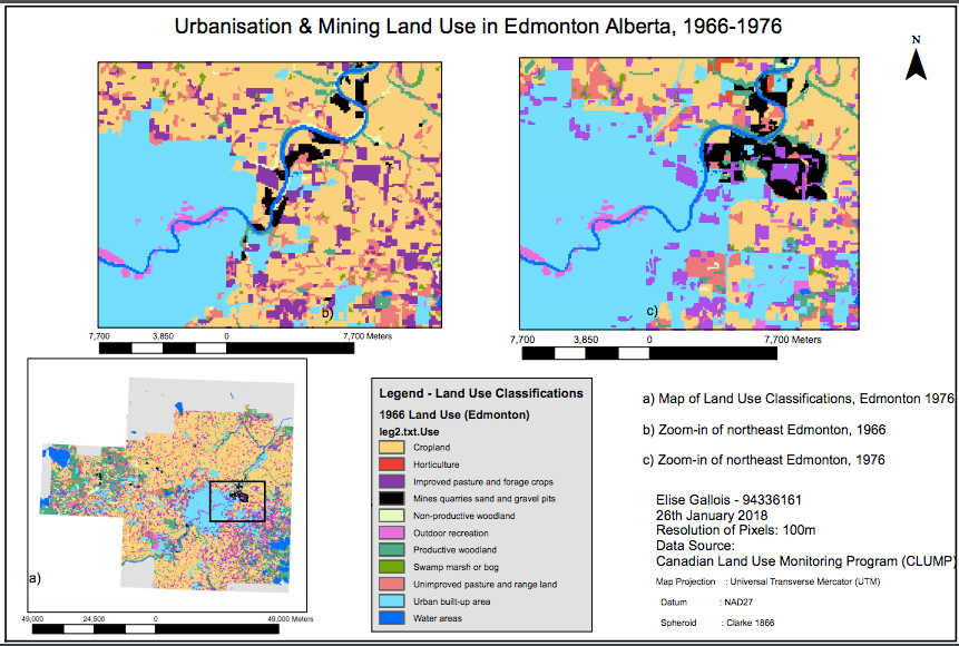
Increased Urban Expansion in Edmonton 1966-1976
Additionally, productive woodland has increased at the expense of unimproved pasture to the northwest and southeast of Edmonton, as can be seen in the map below:
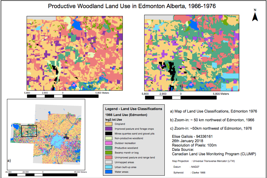
Increased Urban Expansion in Edmonton 1966-1976
Based on the analysis in this report, I believe the following recommendations would be beneficial in increasing our understanding of the described phenomena:
- Further analysis should be pursued to investigate potential correlations between the change in landscape metrics between 1966 and 1976. Multiple regression could determine the extent to which predictor variables such as population change and socioeconomic factors.
- A greenbelt system could be installed to prevent further exponential urban expansion into agricultural land. Furthermore, increasing collaboration with the local government and stakeholders could mitigate future conflict surrounding issues of food sustainability, industrialisation and access to outdoor recreation.
- Further research could be pursued on the increased prevalence of forest edges and the possibility of increased vulnerability to invasive species.