In this lab, the Crimestats analysis software was used to analyse the spatial and temporal distribution of a number of crimes between January 2005 – March 2006 in Ottawa (ON): vehicle theft, breaking and entry (residential), breaking and entry (commercial). A Moran’s Correlograms (below) shows that the spatial autocorrelation of breaking and entry (residential) incidents is highest of the crimes, followed by Vehicle thefts and break and entry (commercial) incidents. Additionally, these all appear to share spatial autocorrelation with the population variable.

The Nearest Neighbour Analysis Index (below) indicate that the crime with the highest level of spatial clustering is breaking and entering (commercial), while the lowest is breaking and entering (residential). This is unsurprising considering the presence of commercial hubs in urban areas.

1st, 2nd and 3rd order nearest neighbour risk-adjusted spatial clustering results (below) represent ‘clusters’ within ‘clusters’ of crimes and accounts for population distribution. Thus, the map indicates areas at particular risk of residential breaking and entry crimes, given the population. The areas at risk are in the central downtown area and in other distinct pockets in suburbs and satellite towns.

While we also produced single dual kernel density analysis maps, I found the dual kernel density map to be the most useful as it shows the relative density of breaking and entering (residential) crimes in Ottawa while accounting for population density. The map indicates higher risk in localised pockets downtown in and particular suburbs away from the city centre, with low z-scores likely representing more sparsely populated parts of Ottawa.

The spatial nature of some datasets (for example, Census data) allows us to investigate the extent to which these associates vary in strength and direction across space. The aim of this lab was to model child social skills against a model Geographically Weighted Regression (GWR) model composed of a set of statistically selected independent variables related to the child and to their neighbourhood. Geographically Weighted Regression (GWR) is a spatially resolved statistical form of regression that allows the value of the dependent variable to vary between locations based on the assumption that so too do the values of the independent variables, as the relationship between phenomena are not fixed across space.

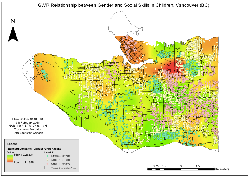
Gender as a predictor of social skills in children

Gender appears to have a notably varied effect on children’s social skills across the cities. In the West End and Mount Pleasant, being a female predicts lower social skills, in comparison to areas of South Vancouver and Hastings where it appears to have a positive impact. The relationship between language skills and social skills is positive across the city, though notably less pronounced in parts of South Vancouver (i.e. South Granville, Shaughnessy and Cambie) where the standard deviation reaches a low of 0.31. Finally, the relationship between parent’s income and social skills is lowest in areas of East Vancouver (i.e. Main and Victoria) with a standard deviation of -1.8, higher in Renfrew (standard deviation of 2.5), though the map indicates a relatively weak relationship between the two variables in comparison to the gender and language skills. The r² values from the model output were plotted as point data and overlaid onto the raster coefficient maps – the highest fit of the models to the data are clustered in central East Vancouver and lowest in areas such as UBC and South Vancouver.

Grouping Analysis:

The ArcGIS grouping tool was used to categorise neighbourhoods of the city with shared characteristics as determined by GWR. This provides a more nuanced view of differences in childhoods across the city than simply ‘east vs west’. This analysis generated the following groups, which were choropleth mapped :

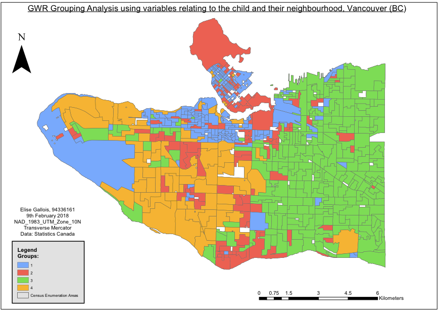
The legend categories 1-4 are detailed below:

1. UBC, Mount Pleasant, West End, Marpole

This area has the lowest % of families that spend 30 or more hours on childcare per week, the lowest number of families >4 and the lowest number of neighbourhood immigrants.

2. Stanley Park area, Strathcona

This area has the highest number of neighbourhood immigrants.

3. East Vancouver

This area the highest number of low parent families, the highest % if families that spend 30 or more hours on childcare and the lowest average income.

4. Kitsilano, Dunbar

This area has the highest income, the highest number of families >4, and the lowest number of lone parent households.

In Lab 2, we used the Fragstats software to analyse land use change around Edmonton between 1966 and 1976. The below maps show the land use maps in the entire study areas for each of the two years, using land use data downloaded from Canada Land Use Monitoring Program (CLUMP) data for Edmonton from the Geogratis website:

1966 Land Use in Edmonton

1976 Land Use in Edmonton

The Fragstats analysis revealed a number of noteworthy changes. One major trend is the decrease in cropland extent as land within this decade was converted to urban land, unimproved pasture, productive forest and mining. Urban areas increased in extent over this decade – both in the city of Edmonton and in smaller settlements, mostly located along the North Saskatchewan river, as can be seen in the map below:

Increased Urban Expansion in Edmonton 1966-1976

Additionally, productive woodland has increased at the expense of unimproved pasture to the northwest and southeast of Edmonton, as can be seen in the map below:

Increased Urban Expansion in Edmonton 1966-1976

Based on the analysis in this report, I believe the following recommendations would be beneficial in increasing our understanding of the described phenomena:

• Further analysis should be pursued to investigate potential correlations between the change in landscape metrics between 1966 and 1976. Multiple regression could determine the extent to which predictor variables such as population change and socioeconomic factors.
• A greenbelt system could be installed to prevent further exponential urban expansion into agricultural land. Furthermore, increasing collaboration with the local government and stakeholders could mitigate future conflict surrounding issues of food sustainability, industrialisation and access to outdoor recreation.
• Further research could be pursued on the increased prevalence of forest edges and the possibility of increased vulnerability to invasive species.