Review: Socio-economics drive woody invasive plant richness in New England, USA through forest fragmentation

 Bibliographic Information: Allen, J.M., Leininger, T.J., Hurd, J.D. et al. Landscape Ecol (2013) Socio-economics drive woody invasive plant richness in New England, USA through forest fragmentation.  28: 1671. https://doi.org/10.1007/s10980-013-9916-7.

The research objectives of this paper are:

  1. To determine the strength and direction relationship between forest fragmentation and woody invasive plant richness.

2. To use selected socioeconomic and environmental factors to explain the land use and land  cover (LULC) in addition to the observed patterns of forest fragmentation .

Building on previous observations about invasive species being more prevalent around the forest edge (in comparison to the forest core), the authors attempted to assess this theory in New England in the United States. Additionally, because urban centres are rapidly developing in this area, they wanted to determine the extent to which certain socio-economic (e.g. single family housing) and environmental (e.g. elevation) factors can be used to predict forest fragmentation change.


This research used a wide range of data and technological processes :

  1. three categories of data including landscape response data and species richness data (collected from NOAA and citizen science initiatives), and socioeconomic data (from the US Census)
  2. Methods of satellite data geoprocessing and LUCL classification (GIS), spatial analysis and statistical models

Hierarchical bayesian modelling was used to predict changes in forest fragmentation and land use class distribution by each socio-economic and environmental variable given the properties of the rest of the data, with the outputs (such as spatial random effects) displayed on ArcGIS. It was evident from the model that socio-economic factors (driven by population) do explain forest fragmentation patterns in the region. Additionally, invasive species richness data was mapped and statistically analysed to reveal that, as expected, woody invasive richness is significantly and positively associated with forest edge areas and significantly and negatively associated with forest core areas – thus, future fragmentation is likely to increase the probability of woody invasive species spread.

What worked well? The methodology was robust and highly replicable – the method can be used the model forest fragmentation patterns in other regions. The citizen science element allowed for easy data-collection and likely engaged many non-expert volunteers in local ecology. However, due to the scarcity of volunteers in northern New England, this method meant richness data was not evenly distributed.

For these reasons, we rated this paper 8.5/10.

Review: Modeling fire and landform influences on the distribution of old-growth pinyon-juniper woodland

Reference: Weisberg, P. J., Ko, D., Py, C., & Bauer, J. M. (2008). Modeling fire and landform influences on the distribution of old-growth pinyon-juniper woodland. Landscape Ecology, 23(8), 931-943.

I chose to review this presentation by Bowen Lan and Leian Cindy Chen because I am interested to learn more about the relationship between fire and woodland, particularly in the Western US where we are seeing a rising frequency of forest fires, and how this trend is influences the distribution of species across the landscape.

Old-growth Pinyon and Utah juniper forests are commonly distributed throughout the Western US. A key knowledge gap is the reason for the lack of diversity in the area –  is this driven by fire history? The authors created models of old growth distribution, taking into account topography and fuel in order to address the following research objectives:

  1. Determine which fire risk component is most strongly associated with old growth distribution.
  2.  Assess the strength of the association between fire and spatial distribution in pinyon-juniper woodland.

The study site was a watershed area in Nevada. The authors mapped the current distribution of old-growth woodland and made models for predicted old growth distribution using cellular automated simulation to predict old growth distribution by adding fire and topographic variables to their models.

Model 1:

In ArcGIS, the authors modelled both the spatial variability in fuel loading in addition to the topographic convergence and solar radiation indices. These indices were z-standardisted into the three categories: low, moderate, and high. Patterns were then identified, including the observation that upper slope sites have a low probability of fire development due to the low fuel availability and greater exposure.

Model 2: 

The authors also modelled the topographic barriers to the spread of fire, using GIS to identify and mark the locations of ridge lines, proximity to rock outcrops, and rating on the wind exposure index (which combines meteorological and topographic data).

Model 3:

The final model was a combination of fuel loading factors and topographic barriers (thus, a mix of biotic and abiotic variables).

Ultimately, it was determined that the spatial distribution of fuel material influenced the agre structure of the landscape to a greater extent than topographic barriers.

Bowen and Cindy gave the study a 7/10 because the models were novel and robust and could be applied to future spatial distribution studies, however landscape dynamics are complex so they believe the authors could have incorporated more independent variables into their models.


Lab 1 – Heart Disease HotSpots

Heart Disease Rate Hotspots in the Southern USA 2016

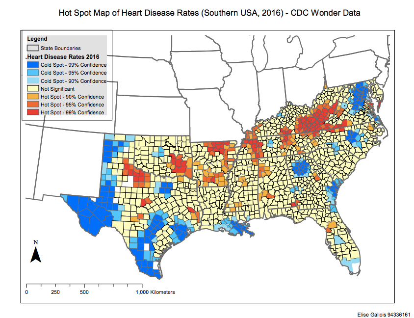
Map 1: Hotspot analysis of Heart Disease in Southern USA, 2016

This map represents hotspots of Heart Disease in the Southern US States in the year 2016. The input data was heart disease rate (which was derived from the Centre for Disease Control and Prevention. The red polygons represent the highest rates of heart disease by county, and the blue polygons represent the lowest rates of heart disease by county. The legend outlines the level of statistical significance (from the Getis-Ord Gi* statistic) and the ‘hot’ and ‘cold’ hotspots visually represent significantly high or low occurrences of heart disease by county, with non-significant occurrences by county represented in yellow. The analysis was conducted using the HotSpot analysis tool on CDCP data in ArcGIS.

There are clusters of ‘hot’ hotspot counties (99% significance) throughout Oklahoma, in Southwest Georgia, West Virginia, East Kentucky and Northwest Tennessee in 2016, indicating that these counties have a significantly high rate of heart disease in comparison to the norm. Each of these clusters is bordered by 95% confidence and 90% confidence ‘hot’ hotspots. ‘Cold’ hotspot clusters (95-99% significance) can be found in West and South Texas, North Carolina and South Louisiana, in addition to smaller clusters in patches on the east coast. Again, these clusters appear to be bordered by ‘Cold’ hotspots of 95% and 90% significance. It could be generally stated that there are more counties with significantly high heart disease rates in the interior, and more counties with significantly low heart disease rates at the coast. The majority of counties show no statistical significance, although it should be noted that there are a number of counties with missing data (particularly in western Texas).

Further analysis could involve determining the extent to which these patterns are influenced by variables such as population density, socio-economic indicators and mobility, perhaps through spatial autocorrelation. This data could be useful to healthcare policy-makers in targeting heart disease treatment and preventative measures to the counties that show a significantly high heart disease rate.


Class 4: Statistics

Regression

Regression is the search for explanatory relations between a dependent and an independent variable (or variables, in the case of multiple regression). Linear regression is used in cases where coefficients are linear (for example, using Ordinary Least Squares analysis, or OLS). OLS models can be fixed where errors are normally distributed and independent from one another, and the data are sourced from independent random samples.

In GIS, regression can be used spatially by applying tools such as OLS to map varying degrees of strength of the relationship between the dependent and predictor variables. Competing models can be selected by finding the highest r2-value (how much of the variance of the data can be explained by a predictor variable?) and the lowest AIC value. Thus, it is possible to use statistical tools in ArcGIS to fit a model that incorporates spatial autocorrelation (see Class 2).

Application

If we have spatial data for variables that we suspect might be related, we can use regression methods to investigate the direction and strength of those potential relationships. In landscape ecology, for example, researchers may wish to investigate the relationship between biodiversity loss and processes such as forest fragmentation.

Potential Caveats

While regression is a powerful tool in spatial analysis, there are some issues that can arise in a model without careful consideration. For example;

  1. Multi-collinearity: the existence of correlation between multiple predictor variables, which should ideally be independent of each other.
  2. Omitted Variables: cases where important predictor variables are excluded from the model.
  3. Endogeneity: cases where the dependent variable actually causes changes in the predictor variable, in comparison to the expected model.


Class 3: Understanding Landscape Metrics

Class 3: Understanding Landscape Metrics

Spatial patterns, ecological processes and interactions across ecosystems are key concepts within landscape ecology. Landscapes, for example, are considered to be inherently heterogeneous. Process-based research requires analysis of landscape pattern (also referred to as form) – what underlying processes determine the pattern we see in the landscape? On school of thought suggests that the patterns we see on the map are only one of many potential landscape patterns that may have materialised by such processes.

So what statistical tests can we use to determine whether the observed pattern has been generated by a hypothesised process?

We assume that where things are, especially in relation to other things, will have particular consequences. We can use spatial autocorrelation (see Class 2 notes) to determine the extent to which the variables are distributed in any meaningful pattern, and are associated with each-other. Types of spatial autocorrelation include clustering, dispersed and random.

Pattern Types:

  • Patterns generated from a response to environmental conditions (i.e. elevation) are known as first order processes.
  • Patterns generated from a response to the distribution and interactions between other variables (i.e. presence of predators) are known as second order processes.

Process Types:

Stationarity

Stationary assumes that the process regime stays the same, and that processes aren’t inherently direction (the processes are isotropic as opposed to anisotropic).

  • Stationary processes are processes that do not change (or drift) over space:
  • A process that has no variation in intensity over space are known as first-order stationary.
  • A process that has no interaction with other variables across space are known as second-order stationary. For these processes, you might use kriging.

There are a number of abiotic (i.e. climate, topography, soils) and biotic (i.e. disturbance, competition, distribution of keystone species) factors operating within a landscape. It is also important to consider human land use impacts on habitats. Landscape patterns are the result of a combination of different processes acting on multiple scales.

Creating and Maintaining Heterogeneity

There are three causes of spatial patterning:

  1. Local uniqueness
  2. Phase differences caused by disturbances
  3. Dispersal

Landscape metrics include the number of cover and class types, texture patterns, compaction of patches, whether patches are planar or linear, and other the patches are complex in shape. However these are difficult to quantify and prove significant.

Class 2: Why is ‘geography’ important?

This class outlined the importance of scale (the spatial domain) to any research with a geographic focus. Different scales will have different degrees of influence on a pattern or process, and explanatory models are inherently scale-dependent.

Spatial Statistics

Spatial Autocorrelation: This is a spatial statistic which determines the extent to which a quantity on of one spatial. If positive, the variables are visible in clusters and if negative, they will be visible as equidistant. The non-random distribution of organisms on the planet means that in fields such as ecology, the research will have an inherently spatial dimension.

Kriging: This is a geostatistical interpolation tool which applies a smoothing function  to fitted values.

Moran’s I value: This is a weighted product moment correlation coefficient – effectively, a similar tool to Pearson’s-r, but suitable for spatial data.

Modifiable Areal Unit Problem (MAUP)

MAUP is an issue in all spatial analyses consisting of the uncertainty about what constitutes the objects of spatial study, and the introduction of bias dependent on the scale selected for research. Running statistics on the same data using different scales can generate different statistics – how can we be confident that we have selected the correct spatial domain? This is especially problematic considering that we usually receive data on only one scale, so we have no flexibility in altering the scale and comparing statistics.

MAUP also involves the issue of groups being used to represent the behaviours of an individual (the ecological fallacy) and individuals being used to represent the behaviours of a group (the individualistic fallacy).

Simpson’s Paradox

This is the issue that multiple variables can statistically correlate, but are actually commonly influenced by a shared variable that may not always be captured in analysis. For example, while the number bars and churches in cities appear to be correlated, they are in actuality influenced by the size of the overall population. Thus, it is important to critically consider the potential for misinterpretation that may arise from statistical analysis (such as spatial autocorrelation).

Class 1: Introduction to GIScience in Research

GIScience can be applied to any field in which geography is an important consideration. Where processes operate across space, spatial analysis can be applied to inform academic theory and management. This course is designed to outline the analysis tools that can be applied to the following three topics:

Landscape Ecology

Landscape Ecology is a branch of Ecology which focuses on the extent to which ecological processes are influenced by the structure of landscape, encompassing the processes and interactions by and between organisms in the context of their physical environment. The scale of these interactions is generally smaller than the distribution of the overarching pattern. The link between these interactions and the structure of the landscape is ripe for spatial analysis using GIScience

Crime Analysis

Geography can be a useful lens through which to investigate crime. In the context of space, factors such as population, mobility, politics, economics and culture can be integrated to investigate criminal patterns. The use of spatial analysis alongside theories in the field of criminology can ultimately assist in the development of administration and our understanding of the relationship between criminal activity and place.

Health Geography

Healthy Geography can be studied on a number of scales and from a range of perspectives. Three of the dominant topics in this field are disease ecology, health care delivery and environment and health. The spatial analysis of these topics under different geographical perspectives can inform the effective deployment of healthcare services where they are most necessary.