Monthly Archives: March 2018

Lab 3: Geographically Weighted Regression

The spatial nature of some datasets (for example, Census data) allows us to investigate the extent to which these associates vary in strength and direction across space. The aim of this lab was to model child social skills against a model Geographically Weighted Regression (GWR) model composed of a set of statistically selected independent variables related to the child and to their neighbourhood. Geographically Weighted Regression (GWR) is a spatially resolved statistical form of regression that allows the value of the dependent variable to vary between locations based on the assumption that so too do the values of the independent variables, as the relationship between phenomena are not fixed across space.

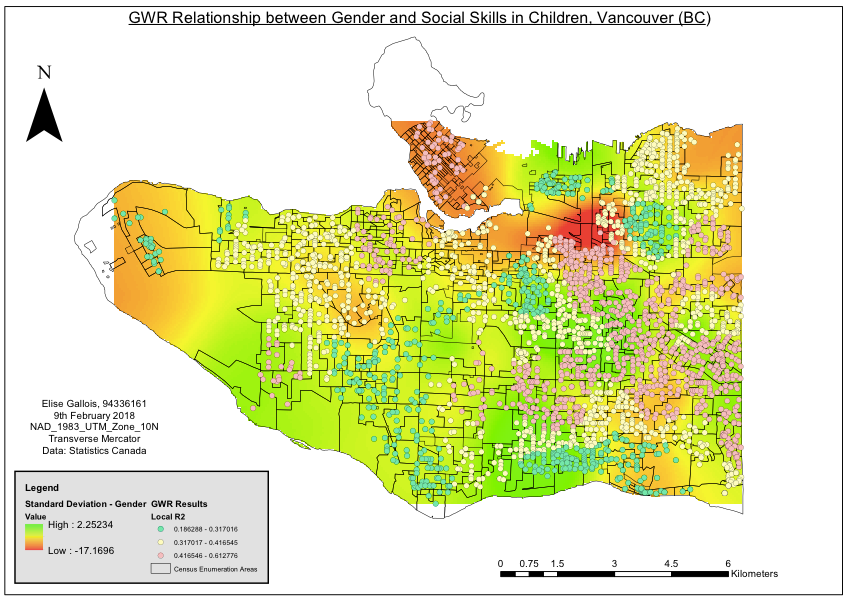
Gender as a predictor of social skills in children

Gender appears to have a notably varied effect on children’s social skills across the cities. In the West End and Mount Pleasant, being a female predicts lower social skills, in comparison to areas of South Vancouver and Hastings where it appears to have a positive impact. The relationship between language skills and social skills is positive across the city, though notably less pronounced in parts of South Vancouver (i.e. South Granville, Shaughnessy and Cambie) where the standard deviation reaches a low of 0.31. Finally, the relationship between parent’s income and social skills is lowest in areas of East Vancouver (i.e. Main and Victoria) with a standard deviation of -1.8, higher in Renfrew (standard deviation of 2.5), though the map indicates a relatively weak relationship between the two variables in comparison to the gender and language skills. The r2 values from the model output were plotted as point data and overlaid onto the raster coefficient maps – the highest fit of the models to the data are clustered in central East Vancouver and lowest in areas such as UBC and South Vancouver.
Grouping Analysis:

The ArcGIS grouping tool was used to categorise neighbourhoods of the city with shared characteristics as determined by GWR. This provides a more nuanced view of differences in childhoods across the city than simply ‘east vs west’. This analysis generated the following groups, which were choropleth mapped :
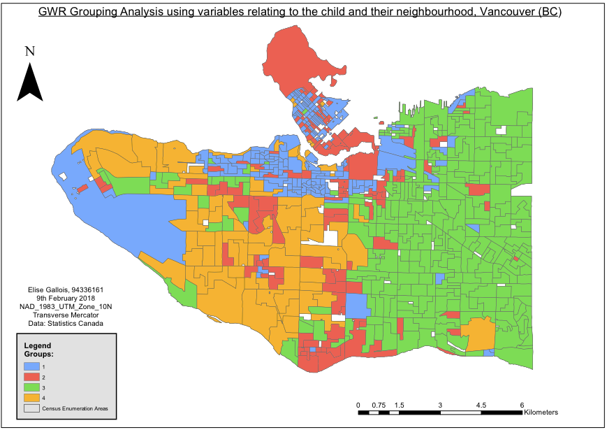
The legend categories 1-4 are detailed below:

  1. UBC, Mount Pleasant, West End, Marpole

This area has the lowest % of families that spend 30 or more hours on childcare per week, the lowest number of families >4 and the lowest number of neighbourhood immigrants.

  1. Stanley Park area, Strathcona

This area has the highest number of neighbourhood immigrants.

  1. East Vancouver

This area the highest number of low parent families, the highest % if families that spend 30 or more hours on childcare and the lowest average income.

  1. Kitsilano, Dunbar

This area has the highest income, the highest number of families >4, and the lowest number of lone parent households.


Class 7: GIS & Crime

Instead of merely a function of temporal and socioeconomic aspects as a predictor of criminal activity, crime can also be considered as a geographical phenomena. Environmental criminology incorporates the idea that crime is influenced by our lived environment.

Crime Geography Theory

  • Routine activity theory: individuals with a motivation to commit a crime, a suitable target, and the absence of a capable guardian. 

Routine activities occur in space, as do ‘nodes’ of activity (places of residence, school, work and leisure facilities. Furthermore, transportation effects the location of a crime which is especially visible when you compare between ‘walking cultures’ and ‘car cultures’.

  • Rational choice theory: criminal activities are a result of the individual making what they believe to be a rational and prudent decision to commit a crime.

What are the rewards against the chances of getting caught? The individual might conduct a cost benefit analysis, and the risk might not be homogenous across space.

  • Crime pattern theory: criminal activities are tied into people’s everyday activities

Crimes occur where the daily activities of victims and potential criminals intersect.

Spatial Crime Analysis Types

Geographical profiling is a tool that has been used to exploit the geographic nature of serial criminal offenders to predict the probably location of the next offence. This analysis can incorporate whether the criminal is a commuter (they travel to commit a crime) or marauder (they commit crimes in their own neighbourhood).

Crime Analysis Applications

  • Intelligence analysis investigates organised criminal activity with the aim to link people with events and property via social network analysis.
  • Criminal investigative analysis is the (largely retrospective) study of serial criminal activities with analysis alongside physical, socioeconomics, psychological and spatial variables.
  • Tactical crime analysis incorporates recent criminal incidents and potential criminal activity to investigate trends in criminal activities and identify key suspects.
  • Administrative crime analysis looks at the findings of crime analysis research in the context of legality, politics and practical considerations.

Class 6: GIS in health geography

Epidemiology is, broadly, the investigation of health or disease conditions, causes and distributions. It is the study of health and population. There are a number of mechanisms by which GIS analysts can aid this branch of medicine:

Spatial epidemiology is about describing and analysing disease risk in relation to space. It has been developed in recent years as a function of geo-referenced health data availability, in addition to advancement of the capabilities of GIS and statistical technology. Small area analysis is preferred because of particular correlating relationships between social and environmental variables and health outcomes (i.e. Geographical correlation studies). Important internal details would be lost using a large-scale analysis framework. An issue with small-scale studies is spatial misalignment whereby data might be available in two different spatial units (i.e. polling districts vs dissemination areas), in addition to uncertainty resulting from changing qualities of population datasets, and metrics which are difficult to measure such as population movement. Best practises in spatial epidemiology include allowing for spatial heterogeneity, using well defined population groups, use consistent data (i.e. from surveys) and allow for both latency times and population movement.

Environmental hazards can also be analysed using GIS. This involves investigating the influence of environmental variances (such as the spraying of DDT) on health risk in particular areas, considering the differential exposures of communities to harmful substances or diseases. Historical data can be incorporated to build on our understanding of the spatial distribution of environmental hazards.

The modelling of health services can take a number of forms. For example, models of public accessibility to health services can be constructed to calculate the extent to which individual communities can easily seek out medical care.

Identifying health inequalities is a particularly valuable outcome of health GIS analysis. Many studies have outlined higher levels of risk of smoking-related disease to individuals in lower socio-economic groups. Furthermore, communities often exhibit inequity in accessibility of healthcare services.

Disease classifications are challenging because they may be the result of multiple causal agents and can have different manifestations among different population subgroups.