Spatial Interpolation:
Most of the data are in points and don’t necessarily overlap in space (e.g. a point with fire incident information but no pest infestation information). To obtain continuous coverage of variables across BC, data need to be spatially interpolated. There are many different kinds of techniques for spatial interpolation: IDW (inverse distance weighted), spline, kriging and others. Each method has its pros and cons.
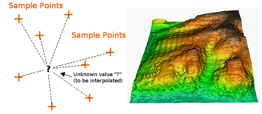
IDW Interpolation [1]
(Here are some simple explanations of the three different techniques from ESRI) IDW uses neighbouring points to interpolate a location’s value. Each neighbour’s weight of influence to the interpolated location is inversely related to its distance to the location. Spline generates a smooth surface by constructing two-dimensional minimum curvatures. Kriging is similar to IDW and Spline in the sense that they are based on the Tobler’s law (relationship decreases with increasing distance). But unlike IDW and Spline, it is based on statistical models. Kriging includes spatial autocorrelation between neighbouring points at distances. In another words, two neighbouring points with exact same distance will be weighted equally in the IDW method but can be weighted differently in Kriging.
Data in this project were spatially interpolated with Kriging (ordinary spherical) because we expect many of the data are highly spatially correlated (eg: precipitation, temperature, wind etc.). Although mountain pine beetle infestation can occur randomly in space, our investigation of the original point data indicates that there is sufficient amount of spatial autocorrelation to justify the use of kriging interpolation instead of a simpler IDW interpolation.
Choosing Spatial Resolution:
The primary attraction of using a coarser resolution for the analysis is the limitation of computational power. There are lots of points/cells considering the size of the area of interest (944,735 km²). However, if the spatial resolution is too coarse, representation of some highly spatially varying elements maybe distorted. For example, temperature and precipitation can be highly variable in mountainous areas due to the complex topography (i.e. micro-climates). This variation maybe lost during the procedure of aggregation that reduces spatial resolution.
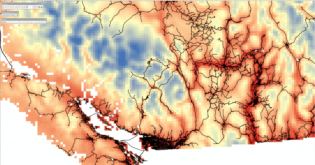
The finest DEM we obtained has a cell size of 77m. The historical climate data from ClimateBC/WNA (PRISM) has a resolution of about 800 m. The wind data from WindAtlas.ca has a resolution of 5000 m. We explored the data with different interpolation resolutions (1001 m, 3850 m and 5390 m) and we are satisfied with spatial resolution of about 5390 m. Below is a raster layer with cell size of about 5400 m.
(Click Map)
Other Data processing:
Original data are clipped with the BC DEM as some data points occurred outside of BC. Some obvious error points are removed by manual identification. For example, the original fire dataset suggests there was a fire in the middle of the Hecate Strait.
Some data are in polygon; for example, the historical fire perimeter. The Arctoolbox “Zonal Statistics” is used to calculate the mean of each topographic or climate parameter in that area covered by the polygon.
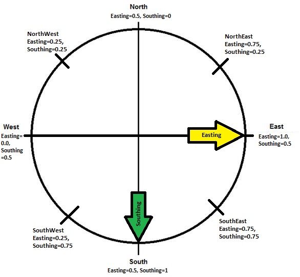
Because aspect generated by ArcGIS is in azimuth angle that can not be used in a linear model, it is split into two variables, Easting and Southing. Each location’s aspect is assigned with an Easting membership (1=East & 0=West) and a Southing membership (1=South & 0=North) using the Fuzzy Membership tool (Gaussian distribution with 0.0001 spread) in ArcGIS. Any aspect can be represented by a combination of Easting & Southing:
Building Multiple Linear Regression Models – Transformation & Model Choosing:
There are 27 variables to start with. Some variables (temperature, slope, pest infestation etc.) are transformed based on simple plotting analysis (with log, reciprocal, square root, power transformation etc.). Predicting variable (fire size in ha) is box-cox transformed in MATLAB 2014a (with Financial Toolbox extension), λ = -0.0929, i.e. Y’=(Y^λ−1)/λ.
SAS 9.4 software is used to choose x-variables for the model, using various model selection methods such as forward, backward and stepwise selections. Two models that meet assumptions of linear regression (linearity, equal variance, normality and independence of observations) are selected for further analysis (See SAS output for more details).
Pairwise Comparisons Between Independent Variables:
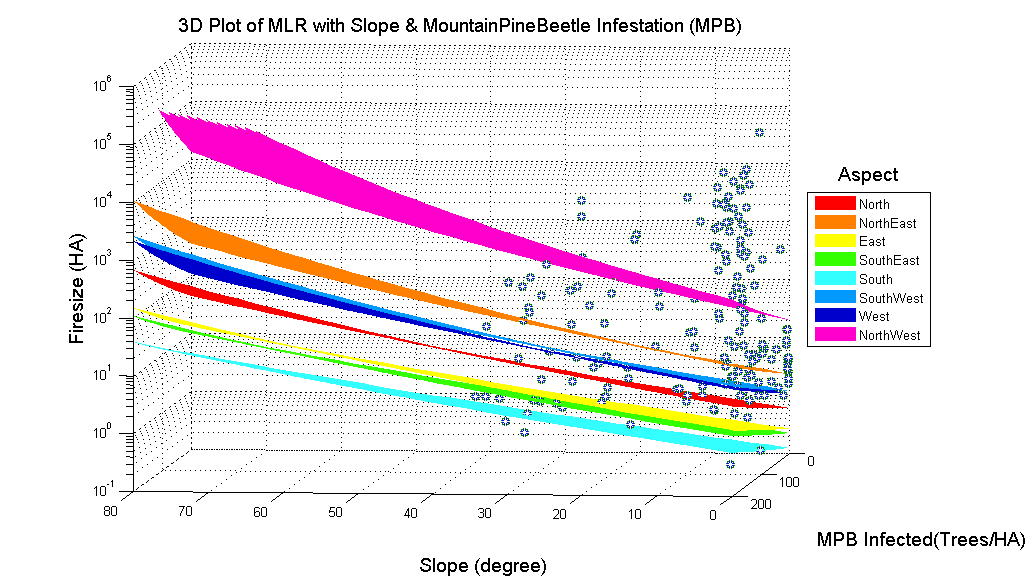
3D surfaces were constructed in MATLAB to compare the influence of each factor on fire size. The range of data of each factor is constrained by observed data.

When comparing a pair of variables, other variables stay constant using the observed mean value. The 8 different aspects are displayed as 8 different surfaces. There are 10 combinations of pair-variables. As an example, below is the Mountain Pine Beetle Infestation and Summer Precipitation pair. The 8 colored layers illustrate the influence of different aspects on fire size. The change of firesize across the observed range of precipitation is more significant than the change of firesize across the observed range of mountain pine beetle infestation, shown as difference in slope.
Fire Spreading Potential Prediction
Using the 2 linear regression models, we predicted the potential fire size in each grid cell in BC. A linear fuzzy membership assigning procedure is performed to evaluate the relative fire spreading potential of each location in the province. The first linear regression model is developed with topographic properties, climatic conditions and mountain pine beetle infestation. The second linear regression model is developed with only topographic properties and climatic conditions (no mountain pine beetle infestation). By comparing these two models, we could evaluate the influence of mountain pine beetle infestation data in predicting fire spreading potential. The difference in R2 between the two linear regression models illustrates how much variation of fire size can be explained by mountain pine beetle infestation.
[1] Documentation QGIS2.2: http://docs.qgis.org/2.2/en/_images/idw_interpolation .png
very cool.