
Data Sources and ASSEMBLY
We used county-level data from various publicly available sources, which were then compiled into an ArcGIS database. Geographic information systems (GIS) shapefiles of US counties and states were downloaded from ESRI and imported into ArcMap software (ESRI, 2018). Data on lung cancer mortality was gathered from the United States Center for Disease Control (CDC) WONDER database from the years 1999 to 2003, which were then averaged into five-year mortality rates for each county. Lung cancer data was specified as malignant neoplasms of bronchus and lung (CDC, 2017). Age-standardized total cigarette smoking prevalence data from 1999 was provided by Dwyer-Lindgren, Mokdad, Srebotnjak, Flaxman, Hansen and Murray (2014). Total smoking prevalence was defined as ‘daily’ and ‘non-daily’ smoking prevalence combined.
Air pollution data was compiled from every monitoring station controlled by the US Environmental Protection Agency (EPA) in the eastern United States. For the purposes of our analysis, the annual (1999) arithmetic mean value of atmospheric particulate matter with a diameter less than 2.5 micrometres (PM2.5) was used as a proxy for all air pollution (EPA, 2000). These points were interpolated to create an air pollution surface using inverse distance weighting, exceeding the study area boundaries where possible in order to reduce potential edge effects (Figure 2.1). Inverse distance weighting was selected because it provides the most accurate visualization of PM2.5 concentration distributions compared to alternative spatial interpolation methods (i.e. trend surface or ordinary kriging methods) (Zhang & Shen, 2015).
Figure 2.1: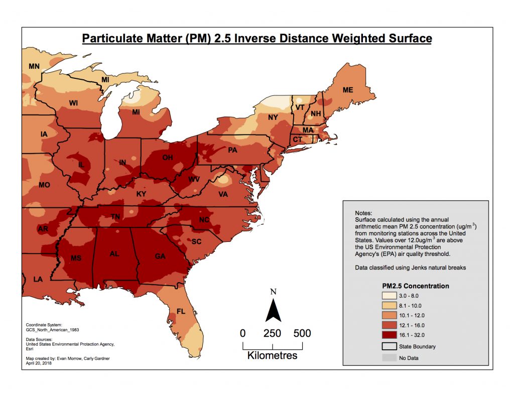
County-level radon risk zones were also provided by the EPA (EPA, 2017). These zones depicted counties predicted to have average indoor radon concentrations greater than 4 picocuries per litre (pCi/L), 2 to 4 pCi/L, and less than 2 pCi/L. Note that Zone 1 is highest risk, while Zone 3 is lowest risk (Figure 2.2).
Figure 2.2: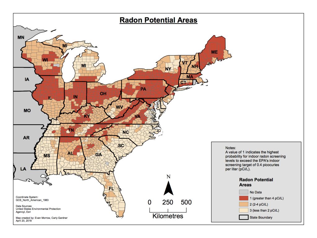
Socioeconomic and demographic data was provided by the US Census Bureau (2000), including median household income (1997), county population (1999), population of racial groups (1999), number of households occupied by renters (2000), and population with a university degree (1990). Populations of numerous racial and ethnic groups were compiled into “non-white” and “white” classes, which were then converted into proportions by dividing by the total county population. Similarly, rented households and populations with a university degree were converted into proportions by dividing by the total number of households or total county population that is 25 years old and over, respectively.