
As OLS is an a-spatial statistical method, it requires data values to be distributed randomly across space and assumes that the explanatory variables exhibit stationarity in their regression coefficients. However, in most cases clustering and non-stationarity are inherent in spatial data, which calls for the use of different spatial statistical methods. Indeed, as Tobler (1970) said, “everything is related to everything else, but near things are more related than distant things.” In both OLS regression results, spatial clustering is evident (see OLS Results). This is why we decided to include geographically weighted regression in our analysis.
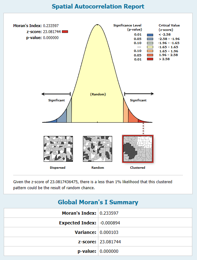
When we ran our OLS regression models in ArcMap, two output surfaces were produced from which we could map residuals. Using the Moran’s I spatial statistics tool in ArcMap, we tested the residuals of both models for spatial autocorrelation. In both cases the residuals exhibited significant spatial autocorrelation or clustering (Figure 4.1). Significant spatial autocorrelation of residuals justified the use of GWR as it signifies clustering and non-stationary within our OLS regression model.
GWR accounts for spatial autocorrelation and non-stationarity by calculating local regression equations for each feature. The output of which can be mapped to view which areas of our study area are best explained by the model (those with highest local adjusted r-squared) and vice versa. For our GWR model we specified an adaptive kernel with an optimal number of neighbours calculated using the corrected Akaike Information Criterion (AICc) bandwidth parameter. The explanatory variables used in the GWR analysis were the same properly specified variables used in the previous OLS regression models.
Unfortunately, when attempting to perform the GWR regression using the explanatory variables determined in Model 2 (which included our smoking prevalence variable) our model experienced severe design problems. As our OLS outputs indicated low variance inflation factors (VIF) associated with our explanatory variables (which test global multicollinearity), it was evident one or more of our variables experienced high levels of local multicollinearity. As this issue could not be resolved through troubleshooting, only Model 1 was used in the GWR analysis.