
Before going into our OLS regression and GWR analysis results, it is important to acknowledge that the results of our analyses are not meant to imply causation. Instead, our regression analyses are used in an exploratory and descriptive manner to look at associations between lung cancer mortality and environmental, social and economic variables. While it may be possible to assume degrees of causation with variables such as smoking prevalence or PM2.5 concentration, we are not asserting that the variables such as low income, proportion of non-white population etc. cause lung cancer and subsequent mortality. Instead, by including these variables in analysis, we hope it will provide insight into the populations which may be experiencing high rates of lung cancer mortality. In doing so, we hope to identify patterns and relationships between lung cancer mortality and underlying socio-economic population characteristics.
Lung cancer mortality rates are significantly correlated with numerous independent variables. The following variables were included in the OLS Model 1: proportion of non-white population, radon risk zone, median household income and proportion of renters. OLS Model 2 included smoking rates, proportion of non-white population, proportion of university educated population, and median household income. Model 1 explained 48% of the observed county-level five-year lung cancer mortality rates (Figure 6.1), while Model 2 explained 54% (Figure 6.2). The VIF for all variables was <5.5, suggesting no global multicollinearity. These results indicate that Model 2 is better correlated with the 5-year lung cancer mortality rate, which is to be expected considering that smoking rates are the leading cause of lung cancer.
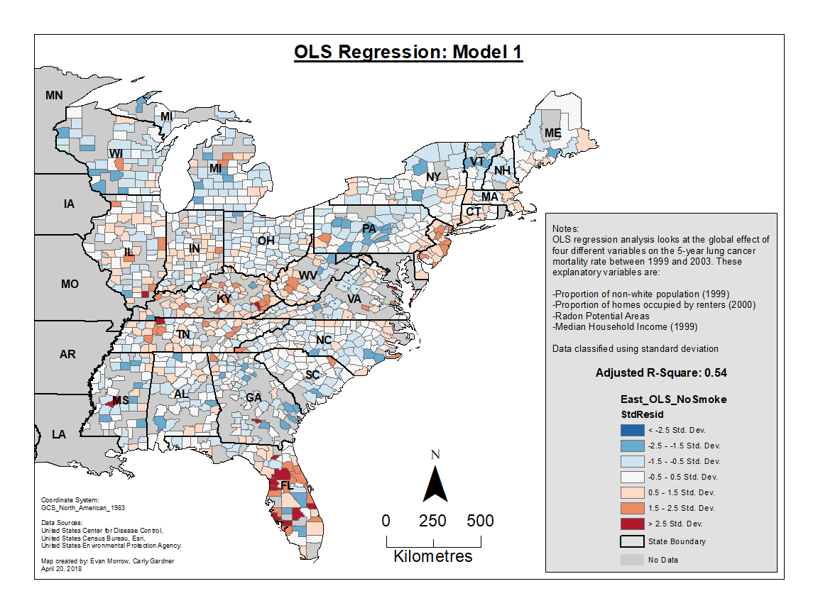
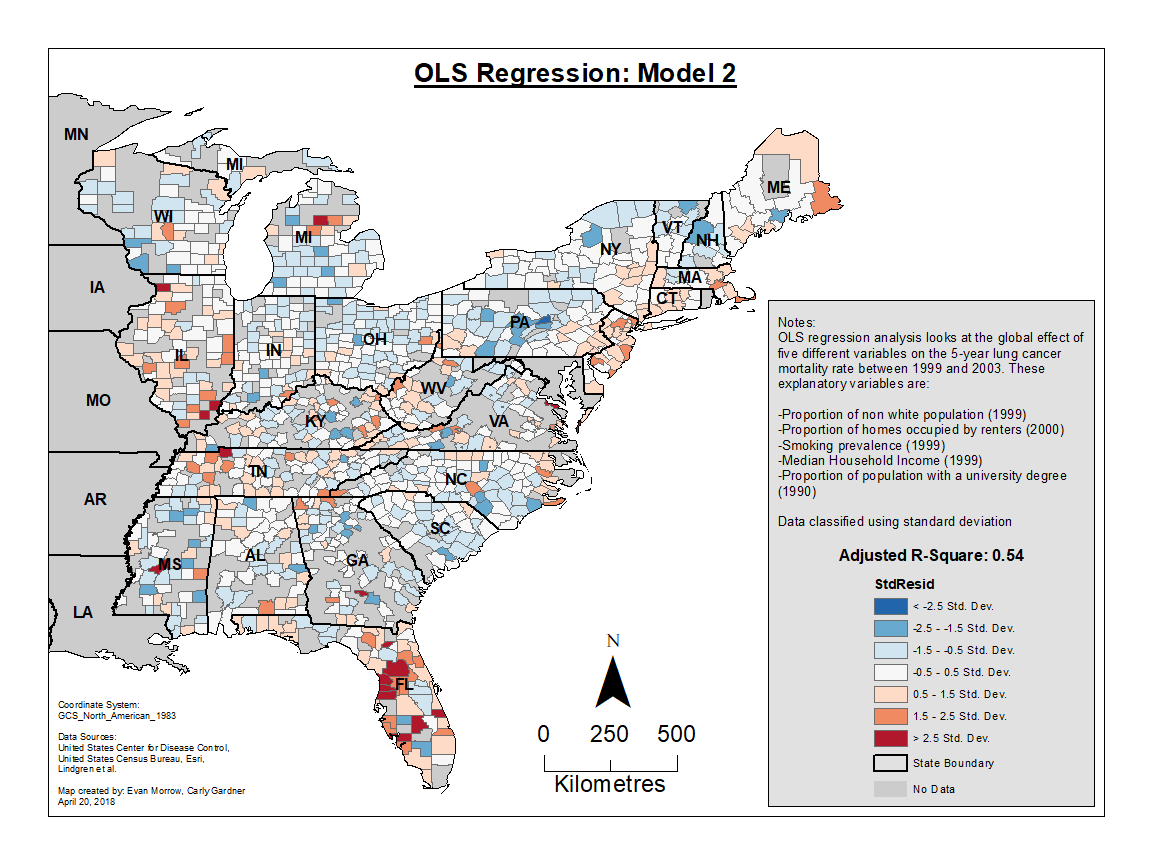
As mentioned in the methodology section, OLS regression only calculates global level statistics that do not take spatial clustering or non-stationarity of explanatory variables into account. Mapping the residuals of both OLS models revealed slight clustering of higher and lower than expected values. For instance, in Model 1 (Figure 6.1), clusters of high values are seen in Florida and the area within and surrounding Kentucky. Similarly, in Model 2 (Figure 6.2), clustering of high values are particularly evident in Florida. Clustering of lower residuals are slightly less pronounced, but can be observed in states such as Pennsylvania. The clustering of residuals in our OLS values indicated that there is variance in regional influences of lung cancer mortality across space. There is more pronounced or significant variability in the relationships between lung cancer mortality and its explanatory variables in these regions of high and low clustering (Florida, Pennsylvania, etc.). Furthermore, as OLS residuals for Model 1 and Model 2 both tested for significant spatial autocorrelation, it is safe to assume that OLS does not fully describe the distribution of lung cancer mortality rates in the eastern United States.