Category Archives: Physically at-risk

The first step we wanted to take in our research is to identify those who were the most physically vulnerable to COVID-19. In this project, we considered age and exposure to air pollutants as the major factors that determine the at-risk population in terms of physical health. The population was divided into four groups: 50-59 years old, 60-69 years old, 70-79 years old and over 80 years old. As for air pollutants, we examined residents’ exposure to fine particulate matter (PM2.5).

To make an integrated analysis on above factors, we conducted Multi-Criteria Evaluation (MCE). CHASS provided the 2016 census data and a shapefile of the transportation network was downloaded from Statistics Canada.

MCE for Age Groups

Location quotients (LQ) were calculated for each factor to identify dissemination areas (DAs) with higher levels of at-risk groups.  LQ is the ratio of the percentage of a given age group in a DA to the percentage of that age group in the whole city of Vancouver. For instance, in DA59150701, there are 530 people over the age of 50, of whom 30 are over the age of 80. In Vancouver, there are 633,125 people over the age of 50, of whom 27,525 are over the age of 80. Therefore, the LQ value of people over 80 years old for this DA calculated is:

LQ = (30/530)/(27525/633125) = 1.30.

If the LQ is greater than 1, the DA has a disproportionately larger share of a particular group of age. We would therefore look at these LQs and normalize those with values of 1 and below to 0. The normalized LQ data were joined to the DA layer and then converted into raster layers for each age group.

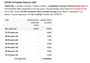
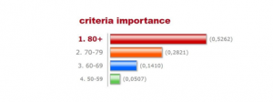
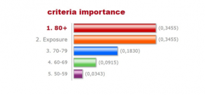
Taking into account the different responses to COVID-19 in different age groups, we weighted it according to the respective mortality rates provided by New York City Health as of April 14 (Figure below). The death rate shows the risk of dying if infected with COVID-19, for a person in a given age group. Weighted importance of each of the four factors was chosen using the analytic hierarchy process (AHP). After comparison of each factor, the weights are as in Figure 2. The final weighted map was then created using Weighted Sum.

The final weighted map was then created using Weighted Sum.

* There was uncertainty involved in this step. The 80+ age group is 11 times more important than the 50-59 age group, but we set the importance index at 9 because it is the maximum on the AHP calculator.

MCE for Age Groups and PM2.5 Exposure

Studies have shown that people with COVID-19 who live in regions with higher levels of air pollution, especially PM2.5, are more likely to die from the disease (Wu et al., 2020). Therefore, we considered long-term exposure to high levels of PM2.5 as another factor in the MCE analysis.

We first created a finer grained surface to show different risk levels with exposure to PM2.5 on a local scale. The major transportation routes included highways and major bus routes were selected from the transportation network data, this layer was then converted into a raster surface.

By using this raster surface, we created a Euclidean Distance surface. Raster calculator was used to normalize the distance surface, and the expression we used was as follow:

( (max value of distance surface – [distance surface] ) / max value of distance surface ) ) *10

The output surface represented the residents’ exposure to PM2.5. It ranged from 0 to 10 and 10 was the closest value to the main road.

To determine the weight of this factor, we referred to the research from Harvard University (Wu et al., 2020), which tells for every 1um/m3 increase in PM2.5 concentration, covid19 mortality increased by 15% (95% confidence interval). Official data shows that from 2009 to 2014, the average concentration of PM2.5 increased by about 1 um/m3 (Government of Canada, 2016) .Therefore, we assume that at least 15% of the deaths of covid19 in vancouver are caused by this increase. The weight of each factor was then recalculated, and the result is shown as below. The final weighted map was also created using Weighted Sum.

* There was uncertainty involved in this step. We assumed that all the roads are weighted equally. A more nuanced representation can be done by using different weights for the different types of roads.