Lab 3
Introduction to CrimeStat
For our final lab we used the CrimeStat program to analyze the spatial distribution of various crimes that occurred between January 2005 and March 2006 in Ottawa. The following is a summary of my results.
Results
Nearest Neighbor Index
The results from this lab for the Nearest Neighbor Index (NNI) analysis of car thefts, break and enter (BE) incidents in commercial areas, and BE incidents in residential areas have been plotted in a graph, shown in Figure 1 (all figures can be found in below). All three types of crime have fairly similar trends and NNI values in general. The NNIs are all less than 1 (meaning there is more spatial clustering than would be expected), and increase fairly quickly for the first five or so nearest neighbor orders and then at a slower rate for higher orders. The overall trend of clustering crimes is to be expected, as there are certain factors that may promote higher crime rates in some areas (for example presence of a bar and alcohol) and factors that may deter crime in other areas (for example presence of a security camera and police patrols). The rate of change in the NNI as order increases is suggesting that crimes are spatially clustering in certain hotspots within the study region.
Moran’s Index
The results from the Moran Correlograms have been summarized in the plot in Figure 2 for each crime type, as well as population within each DA. From this plot, it can be seen that the general trend in Moran’s I values decreases quite steeply until about the tenth distance interval, and from then they remain fairly steady. This indicates that the crimes are more spatially clustered than would be expected simply due to chance, and that larger distances have less spatial clustering of crimes. Though they follow a similar trend in rate of change, the Moran’s I values for the different crime types do differ from the population values (green line on in the plot in Figure 2). Following the same general trend does indicate a link between crimes and population, which is not surprising (with more people there are more opportunities for crime). However, if crime distribution and clustering was only correlated to population, then the Moran’s I values for each crime type would directly mirror the population values. However, clearly this is not what occurs in reality, since there are many factors other than population distribution that impact crime distribution. Factors such as increased / decreased security measures in certain areas, police presence and patrolling, parking lots, and many more will likely also have an impact on how crime clustering occurs across the study region.
The overall results for the spatial clustering from the Moran’s I analysis are slightly different from the NNI analysis. Notebly, the residential BE values from the Moran’s I analysis are much higher than the other crime types, though eventually drop down to a rate similar to that of the car thefts after approximately 15m. This indicates that the residential BEs are much more spatially clustered than would be expected only due to chance, particularly for distances below 15m. In the NNI results, the residential BEs had somewhat significantly higher NNI values than the commercial BEs or car thefts, but in this case a higher values indicates less spatial clustering. This may be due to the somewhat limited number of orders in the NNI analysis, which would limit the results. Furthermore, the Moran’s I method takes into account the incidents as they are associated in DAs, while the NNI just looked at the spatial autocorrelation of individual incidents of crime. Therefore the Moran’s I is a slightly more sophisticated statistical method, and these results may be more accurate to the real world / reliable than the NNI results.
Fuzzy Nearest Neighbor Clusters
In this lab, the fuzzy mode radius was set to 1000m. The map in Figure 3 shows the results of this fuzzy nearest neighbor analysis, with the blue ellipses outlining instances of spatial clustering within the 1000m radius, and the dots indicating the fuzzy mode results. Red dots indicate higher frequency and green indicate lower. For the purpose of displaying the most interesting and relevant results, Figure 3 is a map of the downtown area since that is where the majority of results were located, and an inset map indicates where this is in relation to the entire study region. As can be seen on the map, there are many instances of clustering within 1000m, particularly within the core downtown area. This is expected, since the downtown core is not only the most densely populated, but also likely has the highest concentration of opportunities or driving forces of crime. There are also nearest neighbor ellipses in some areas just outside the downtown core, which are typically residential neighborhoods, commercial areas, or some other type of land use that attracts larger populations (and thus increased opportunities for crime).
Nearest Neighbor Hierarchical Clusters
The map in Figure 4 shows the nearest neighbor hierarchical spatial clustering for the different crime types. While the map in Figure 3 showed first-order clustering, it was non-risk-adjusted. Figure 4 includes these ellipses for reference, but more importantly the ellipses that are risk-adjusted for the first, second, and third order clustering. Risk-adjusted is referring to a correction made to show the relative risk that a person would experience one of the crime types. Clustering the absolute data may lead to misinterpretation, because there may be unknown underlying conditions. The risk was adjusted for using population over 15 per enumeration area, in a secondary surface.
Figure 4 shows similar patterns as found in the fuzzy nearest neighborhood analysis; the downtown core has the most significant clustering, again likely due to the factors that inspire more crime to take place there. The first-order nearest neighbor results that were risk-adjusted appear to be fairly similar to the non-risk-adjusted results of the fuzzy nearest neighbor analysis. In the final third-order cluster, all points are grouped together in one cluster (indicated by the purple ellipse). This gives an indication of a specific area in the entire study region that has the most significant spatial clustering. As previously mentioned, it occurs within the downtown core, and when comparing the Figure 4 to Figure 3, it can be seen that the third-order ellipse encompasses the region that has the highest instances of crime clustered within a certain distance.
Kernel Density (single surface)
The results from the single surface kernel density analysis are presented in a map in Figure 5. The green indicates low values and the red indicates high values. The residential BEs have been included on the map as black dots. This map shows the density of residential BEs, in absolute terms. As seen on the map, there are higher concentrations of residential BEs in specific areas; the downtown core, as well as several other areas outside. These areas outside of the downtown core are likely neighborhoods where there is more residential housing, and therefore more opportunities for residential BEs. The residential BE points external to the red areas are outliers, but are often not surprisingly near major roads, where criminals could easily scope out and access the residential dwellings.
Kernel Density (dual surface)
The results from the dual surface kernel density analysis can be seen in Figure 6, using the same symbology as Figure 5 (though different ranges of values are used for the dual surface kernel density). This map again shows the density of residential BEs, but takes population into consideration, and therefore represents a relative crime density. As such, these results are slightly different from the single surface kernel density results. The relative crime density is important to consider, since it means that the results have been “normalized” for population, and therefore will likely be more accurate in depicting significant results. Overall, the results of this kernel density analysis show that some areas in the study region have higher risk of residential BEs than others, such as the downtown core. Some of the peripheral areas have higher risk of residential BEs than would be expected with the spatial clustering, and this may be due to underlying factors (such as lower income neighborhoods). Some of these areas may also be paths of frequent travel or transit hubs. Crime has been found to be geographically linked to these locations in several studies (Loukaitou-Sideris et al., 2002), since people tend to commit crimes in areas that they are familiar with (such as places they pass and observe during their daily commute to / from work).
Knox Index
In this lab, the Knox Index analysis was used to examine the space-time relationship for car thefts. The results of the Knox analysis are shown in Figure 7, as copied from the text file provided by the CrimeStat program. From these results, it can be seen that more car thefts exist closely in space and time than would be expected due to random chance. Furthermore, it appears that the incidents of car thefts are spatially autocorrelated more so than they are with time. This spatial importance may be due to the spread of specific locations where cars are permitted to be parked within the downtown core, such as within parking garages or along only specific streets. The general trend of crime and time follows the expected results; crime incidents tend to follow hourly patterns, with more crime occuring during mornings and evenings (Felson & Poulsen, 2003). There are also theories such as the “routine activity theory”, which indicates a connection between certain hourly activities and crime rates. However these patterns are impacted by many other factors, such as land use type, season, and population demographics.
Maps & Figures
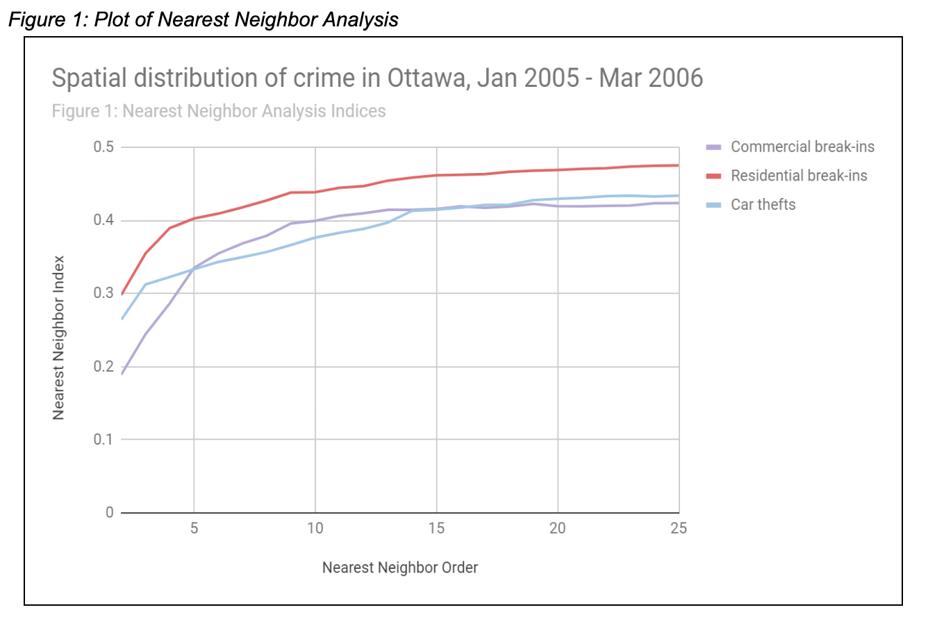
Plot of Nearest Neighbor Analysis
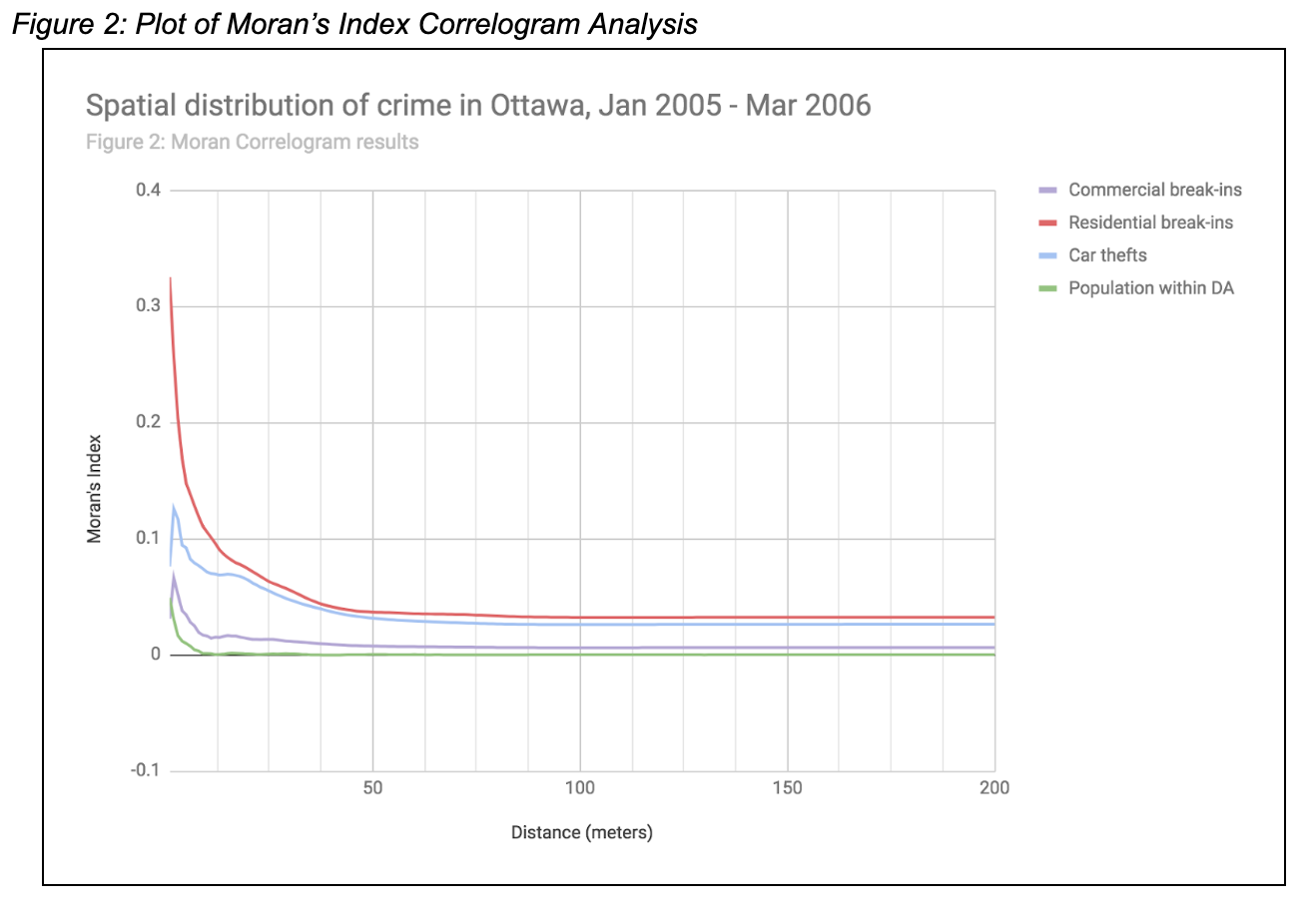
Plot of Moran’s Index Correlogram Analysis
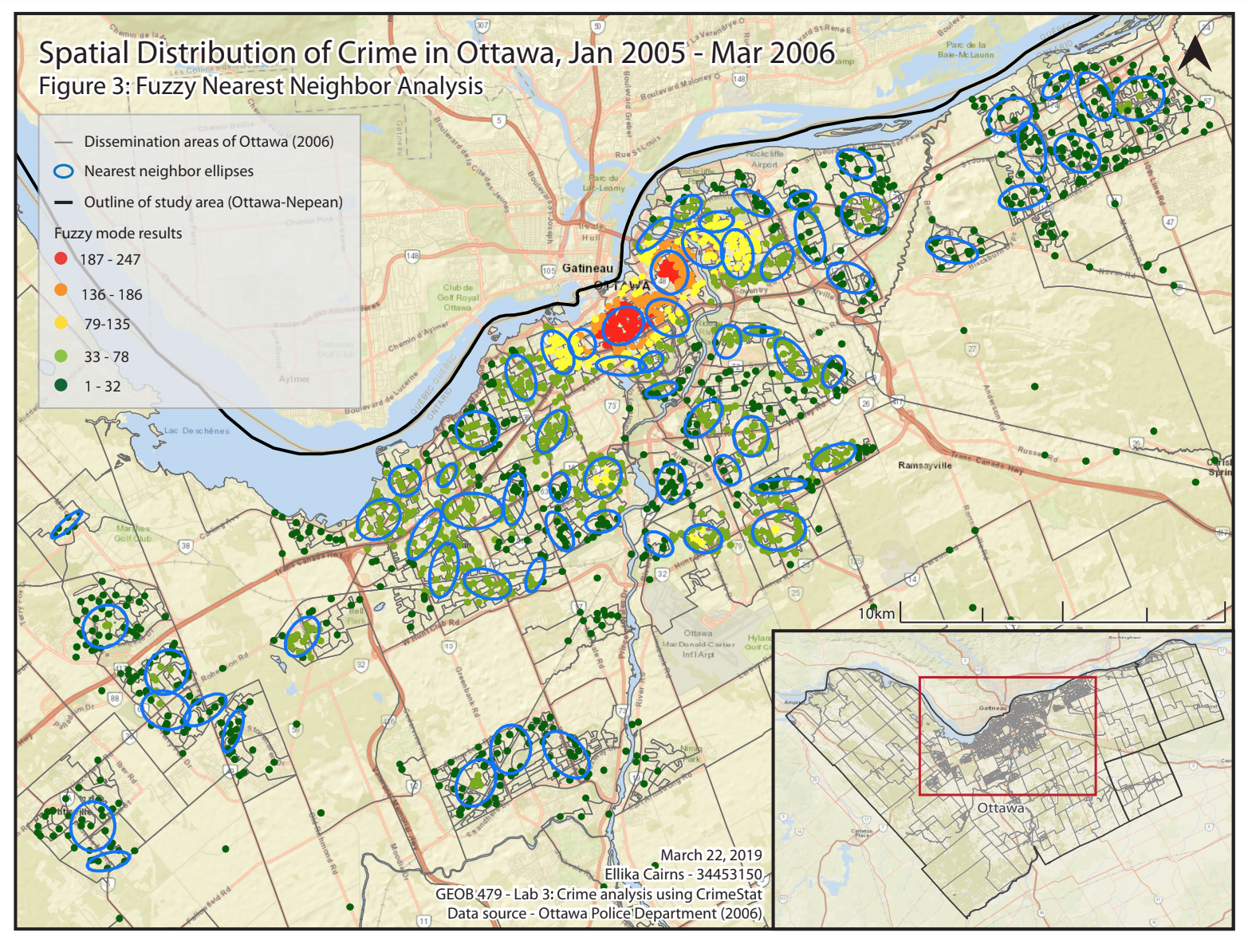
Fuzzy Nearest Neighbor Analysis
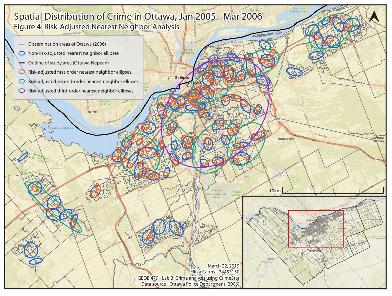
Risk-Adjusted Nearest Neighbor Analysis
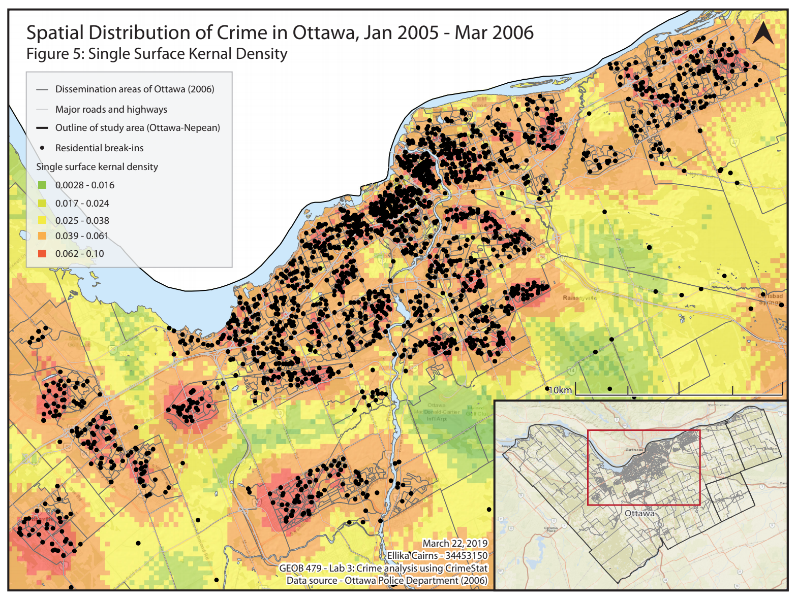
Single Surface Kernal Density
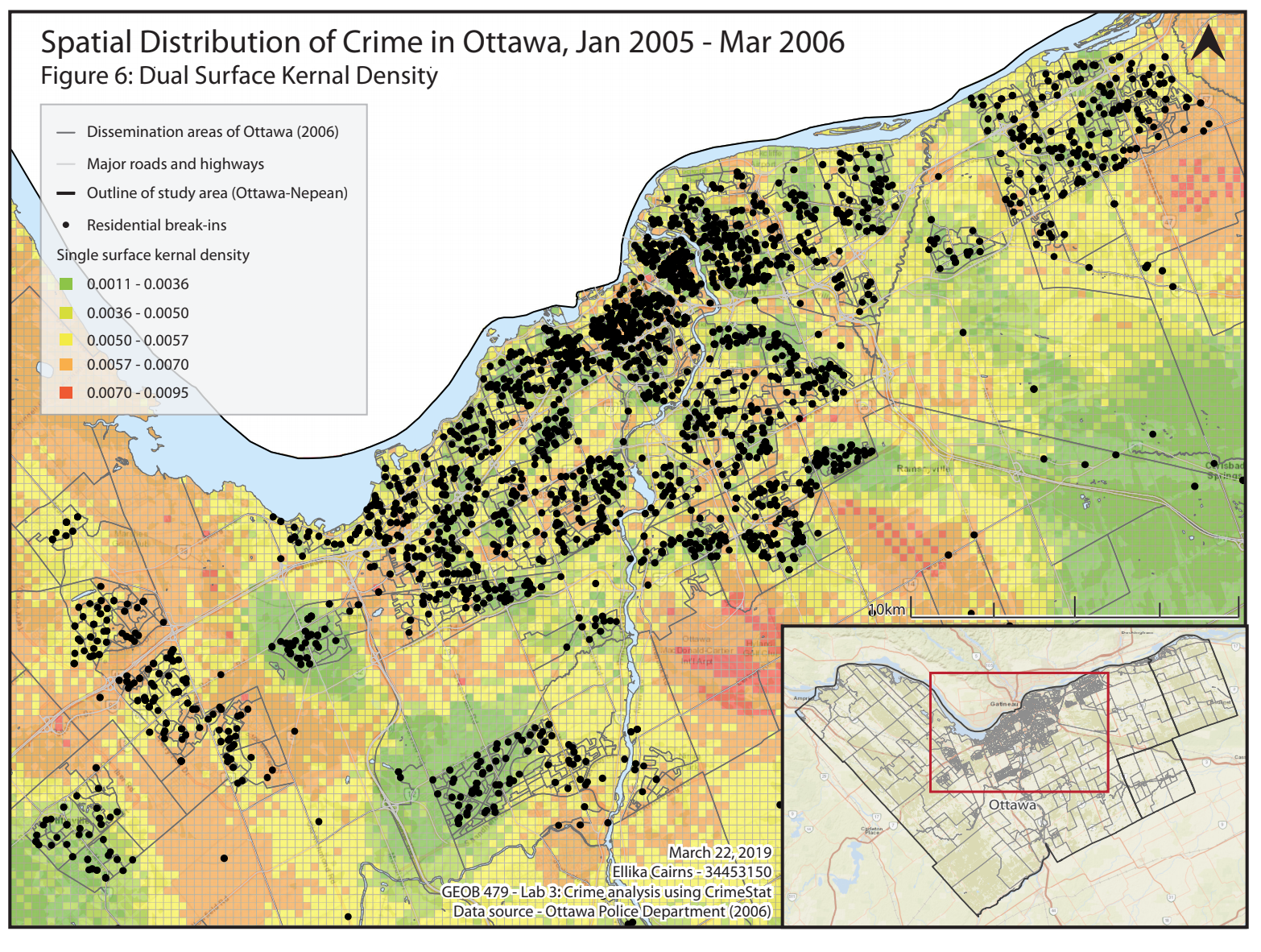
Dual Surface Kernal Density