Category Archives: Electoral Reform & Senate Reform

Proportional Representation cures cancer & wipes out poverty…

It’s been a long time since I wrote a blog post, but impetus has come in the form of Jenny Kwan’s latest “10-percenter”*. (Kwan – unfortunately for me – is the MP for Vancouver East, where I live.) The 10-percenter is on electoral reform, and specifically on the virtues of PR. That’s both understandable and logical given that Kwan sits for the NDP: the NDP bear the brunt of our SMP system’s disproportionality and would likely see their seat share and policy influence increase under PR. If you are an NDP supporter, you ought to support PR on that basis: it’s in your political interest.

Kwan’s pamphlet doesn’t make that kind of straightforward argument, however. Instead, it offers up a rather incoherent and biased comparison of the current electoral system (single-member plurality) and PR. Here’s the full text of Kwan’s pamphlet; I’ve highlighted areas that I examine in greater detail below:

Defenders of the status-quo will likely tell you that proportional voting systems lead to chaos – with endless elections and instability. But the reality is the exact opposite is true.

Canada already has a lot of federal elections. In fact, we’ve had 22 in total since 1945. That makes us more “unstable” than Italy, a country that uses proportional representation and has had just 18 elections over the same period.

Proportional elections eliminate “false majorities” by ensuring no party gets a higher percentage of seats than their percentage of votes. That forces political parties to work together and deliver results in a stable coalition government.

Beyond making our elections fairer and more stable, proportional systems have many other positive impacts on the countries that use them. For example, they tend to have stronger economies with higher surpluses, lower deficits, and less debt.

Countries where parties work together collaboratively are also more likely to tackle two of the biggest issues of our time: climate change and income inequality.

With consultations on democratic reform underway, we have a once in a lifetime opportunity to build a better Canada with fairer elections. We have to get it right.

Let’s start with the incoherent aspects of this argument. The first claim here – if I follow – is that elections are finite in occurrence under PR; that is the exact opposite of “endless elections” is it not? Speaking as a person who prefers to live in a democracy, let me say that I really hope that elections are endless! I guess the question that Kwan’s constituents should pose to her is when will elections end under PR, after one election or two?

The second puzzling aspect of the argument is the comparison that Kwan draws between politically “unstable” Canada and politically stable Italy. Huh?! It’s not only that the data that Kwan presents on this front are highly misleading (see below), but that Italy is precisely the wrong country to bring up when trying to establish that PR’s does not imply political instability. I could see bringing up Austria or Germany or Sweden…. but Italy??

To see how misleading Kwan’s comparison is one needs to appreciate that the metric of political stability in the electoral systems literature (see, e.g., Powell (1982), Lijphart (1999), Farrell (2001, 193)) is not the frequency of elections but cabinet duration. One good reason for this is that the time between mandated elections varies substantially across countries; it’s just 3 years in Australia, for example. Indeed, if I crack open my Stata and upload a data set on elections and cabinets in OECD countries from 1945 onward I find that Australia’s had 27 elections since 1945. Do you think that Australia’s been the least stable OECD country over the post-war period? Me, neither.

So let’s consider how Canada and Italy perform in terms of cabinet stability over the post-war period. (A caveat here is that my data are not well configured to estimate cabinet longevity because they are formatted by election not by cabinet, and while I am exercised by Kwan’s distortions, I’m not so exercised that I’m going to take 45 minutes to reformat my data set). Bearing that caveat in mind, my data (all publicly available on ParlGov) do allow me to present two metrics of cabinet stability:

  1. the average number of cabinets per year, and
  2. the average duration of the initial cabinet, i.e., the cabinet first installed after a general election

My data on Canada cover 70 years, from June 1945 – November 2015.

  • In that period, Canada was governed by 27 cabinets, for an average of .39 cabinets per year.
  • In Canada, initial cabinets (and there’s never been more than 3 in any parliamentary term) have survived an average of 1116 days. This is 61 percent of the maximum time period of 5 years between Canadian elections.

My data on Italy cover 66 years from May 1948 – February 2014.

  • In that period, Italy was governed by 62 cabinets, for an average of .94 cabinets per year.
  • In Italy, initial cabinets (and Italy’s averaged 3.65 per parliamentary term) have survived an average of 524 days. This is 30 percent of the maximum time period of 5 years between Italian elections.**

The difference here is stark. Italian cabinets have been less than half as durable as Canadian cabinets over the post-war period. Thus Kwan’s claim that Italy has had fewer elections than Canada in this period is true, but it’s also incredibly misleading as to which country’s had the more stable governments. (An irony here is that Kwan’s district includes Vancouver’s traditional Italian neighborhood, and so many of her constituents will know exactly what a political basket-case Italy is.)

Now one can certainly debate whether cabinet durability is an informative normative metric; Lijphart (1999), for example, argues that cabinet durability is not necessarily a good indicator of policy-making effectiveness. And we can have too much durability – ossification – as well as too little. But that’s a different argument.

Let me move on to the old “false majority” chestnut. (This critique of SMP just won’t go away – sigh.) It is true that plurality electoral systems occasionally produce elections in which the 2nd-place party in terms of vote share wins the plurality of seats. Note that this is a system-level not a district-level phenomenon. In each district, it’s the candidate with most votes who wins. However, a party’s vote share can be spread in a very inefficient fashion across seats (large majorities in a minority of districts) such that it secures a large vote share but a small seat share. It’s hard – but not impossible – to generate similar distortions under PR; the key is to have a small district magnitude (and many districts) as in Chile’s “binomial” electoral system.

More to the point, PR can easily produce another kind of “false majority”. Imagine that an electorate is comprised of three types of voters with preferences over 3 parties, a, b and c as shown in the table below. Thus voters of Type A prefer party a first, b, second, and c, third. Let’s say that there’s a rough equality between types of voters (so 33% of each), and that they vote sincerely. Thus, parties a, b and c gain roughly equal shares of votes and seats, the electoral system being highly proportional. All parties have equal legislative power under these conditions, and any two can form a majority coalition. Let’s say that a and b form a coalition.

Voter Type

A

B

C

1st preference

a

b

c

2nd preference

c

c

a

3rd preference

b

a

b

Now, on one hand, a coalition of a and b can claim to enjoy the support of a majority because, 2/3 of voters voted for either a or b. On the other hand, the electorate was not presented with a choice over all possible outcomes; they got to vote only for a or b or c – not a coalition of a & b, b & c, or a & c. If voters had been given such a choice, a majority might well have voted for a coalition of a & c given that all a-types prefer a and a & c to b and all c-types prefer c and c & a to b. On this basis, one could argue that the coalition of a and b reflects a “false majority”.

There are two points here:

  1. “False majorities” do not disappear under PR; they just take on a different and less obvious form; these “false majorities’ are not at all inevitable, but they cannot be ruled out ex ante;
  2. Using the concept of a “false majority” to evaluate an electoral system is a dead-end.

I can expand on the second point: One of the central messages of social choice theory is that it’s almost never possible to identify if there exists a coherent and uncontradicted majority in favour of a particular policy or outcome (save in the case of a majority vote over two alternatives). The problem (as I have written and spoken about again… and again… and again) is that the electorate is better understood as an agglomeration of multiple, partly conflicting majorities. The idea is pretty simple: sure, there may exist a majority for policy X and also one for policy Y – but it does not follow that there necessarily exists a majority in favour of both X and Y.

The rest of the claim is no better. The statement that proportional representation “ensur[es] no party gets a higher percentage of seats than their percentage of votes” is not wholly accurate. As Douglas Rae (1967, 134) observed “The prejudice of electoral laws – and here I include even the P.R. systems (my emphasis) – in favor of strong elective parties and against weak ones is very nearly a universal fact of life.”(By strong parties, Rae meant those polling more than 20 percent.)

The reason this occurs is due to a variety of factors; the two main ones are a finite, and typically quite low district magnitude in most electoral systems, and electoral thresholds. If the district magnitude is below 5 or 6 and the electoral threshold in the neighborhood of 5 percent, it’s quite possible for a PR system to deviate significantly from proportionality – and this deviation always favours larger parties. (Certain quotas – like the Imperiali quota — also systematically favour larger parties.)

The last part of the claim, that proportionality “forces political parties to work together and deliver results in a stable coalition government” is not so much false as it is contingent. Certainly, cooperative, stable coalition government is one possible outcome of a PR electoral system; that’s largely the German, Austrian, and Dutch experience.Two other alternative outcomes are possible and widely observed, however.

The first alternative is what Giovanni Sartori (1976) termed polarized pluralism: a pattern of party fragmentation, unstable coalition governments, and policy immobility. This is the French 4th Republic, Italian, Belgian and Israeli experience. The second alternative is minority government; this is Swedish, Norwegian and Danish experience (see Strom 1990).

I actually think this second alternative is the most likely outcome in the Canadian case were we to adopt PR. The fact that Canadian opposition parties have allowed minority governments to form and last indicates that there are significant (unobserved) costs to joining a government and/or bringing down a government in Canada, and possibly significant (unobserved) benefits to being in opposition; else opposition parties would have forced our minority governments into coalition or brought them down immediately. In addition, the structure of the party system facilitates minority government. Let’s say that the Liberals get a plurality of seats under PR and the NDP says “let’s make a coalition.” The Liberals can tell the NDP (and Greens) to go pound sand. What are the NDP going to do? Bring down the Liberals in favour of the Tories or a new election? PR may deliver different seat shares to the smaller parties, but unless the configuration of the party system also changes substantially, it will not necessarily increase their legislative power.

Moving on to our unfair and unstable elections… (Are Canadian elections unstable, marked by widespread violence and irregularities? Perhaps in the 1870s…. but nowadays?) The claim here is that countries that use PR have “stronger economies with higher surpluses, lower deficits, and less debt.”

I am not sure where Kwan gets the statistics to back this statement up because the debate on the macroeconomic effects of electoral systems is far from settled. Lijphart (1999) made similar statements about the superiority of consensus democracies (which use PR) in Chs. 15 and 16 of “Patterns of Democracy”, and in his 1997 EJPR piece he declared: “the results of statistical analysis were clear and almost completely unequivocal. . . Over-all, consensus democracy is superior to majoritarian democracy. I have no second thoughts about these conclusions.”

Lijphart’s evidence was not particularly strong, however; it consisted mainly of a series of bivariate regressions on data up to the 1980s. When Anderson (2001) re-analyzed these data he found that the superior macro-economic performance of consensus democracies disappeared once one controlled for corporatism and central bank independence. In fact, controlling for these two factors (which are not themselves due to the electoral system), Anderson found that consensus democracies had higher rates of inflation and unemployment than majoritarian democracies. These results are consistent with work by Rogowski and Kayser (2002) that finds that price levels are higher in PR systems. Related work by Bawn and Rosenbluth (2006) finds that government spending grows in line with the number of parties in government. That said, Iversen and Soskice find systematically less economic inequality under PR.

The reality is that one could line up literature on both sides of the claim that PR is good / bad for the economy.  My own view is that the electoral system probably has only a small effect on economic outcomes. Other, more fundamental institutions – the rule of law, constitutional limitations on government – probably have a greater impact in the sense that for a society that gets these fundamentals right the electoral system probably doesn’t really matter much. Conversely, get these fundamentals wrong, and changing the electoral system is unlikely to make a damn bit of difference.


* A “10-percenter” is a newsletter that an MP can send to 10% of her constituents on the federal government’s dime.

**OK, so these are not median survival times from a well-specified Cox Proportional Hazards model, and as such they may suffer from right-censoring.  BUT 1) any right-censoring probably understates just how much more stable Canadian cabinets have been relative to Italian cabinets, and 2) this blog is not intended to be a statistics symposium, in any case.

Aside

Just a few off-the-cuff thoughts on recent parliamentary events. I loved – LOVED – the procedural trickery that the NDP & Conservatives pulled on the Liberals on Monday involving bill C-10.  The substance of what transpired was this:  1) Alexandre … Continue reading

Representation, Accountability and Electoral Systems

I was recently (kindly) invited by the Canadian Study of Parliament Group to talk about electoral systems and electoral reform.  Here’s what I contributed. A  bit pessimistic, perhaps, but mainly just a review of some literature on representation, accountability, and electoral systems.

INTRODUCTION

Ideally, government is representative and accountable, representative in the sense that its policies align with citizens’ interests, and accountable in the sense that it is answerable to citizens for its conduct and responsive to their demands.  The electoral system plays an important role in determining how representative and accountable a government is in practice.  Yet, it is tremendously difficult to identify an optimal electoral system, that is, one that maximizes both representation and accountability. This is because much research shows that electoral systems that advance representation tend to do so at the expense of accountability, and vice versa (Horowitz 2003).

The trade-off between accountability and representation is often portrayed as a fundamental obstacle to identifying an optimal electoral system, but any such trade-off is not really what prevents us from identifying an optimal electoral system.  It is rather that we can neither i) reliably identify more or less representative electoral outcomes, nor ii) rely on repeated elections to hold incumbents to account.

THE REPRESENTATION-ACCOUNTABILITY TRADE-OFF

Representation

One can appreciate the effect of the electoral system on representation by recalling Downs’s (1957) model of electoral competition.  The two parties in Downs’s model appeal to voters by altering their policy positions.  The well-known result of the model is that both parties converge on the position of the median voter, who then randomly supports one of the parties to give it a majority. If we take as a metric of representation the policy distance between the median voter and the median legislator (this is called congruence), the result is perfectly representative.

Few real-world elections feature exactly two parties, and once more than two parties inhabit Downs’s model one or more of the parties may benefit by diverging from the median voter.  This has less to do with the electoral formula (plurality or proportional representation (PR)) than the district magnitude (Cox 1990).  Even so, Figures 1a and 1b convey how parties tend to arrange themselves under plurality or PR, respectively (see, e.g., Powell 2000).  In Figure 1a, C takes up a position to the right of the median voter in the hope that A and B will split the vote to the left of the median voter so that C can secure a plurality of votes on the right.  In Figure 1b, A, B and C distribute themselves evenly about the median voter’s position.

Figure 1a & b

The representational consequences of these two stylized elections are quite different.  If C were to win the plurality election in Figure 1a, there would be a substantial gap between the median voter and the majority party, C.  There is no outright winner in PR elections, and in theory A, B, and C ought to arrange themselves in Figure 1b such that each obtains an equal share of the vote (else each would have cause to adopt a somewhat different position).  This would result in legislature in which A, B and C have equal seat shares, and in which the median party (B) is therefore located exactly at the median voter’s position.  In terms of congruence, the PR result is highly representative.

Accountability

Powell (2000) argues that electoral accountability exists when i) there is clarity of responsibility for political outcomes, and ii) voters can effectively sanction those responsible for those outcomes.  Plurality electoral systems tend to score highly on these criteria for two reasons:

  1. Plurality electoral systems tend to produce single-party majority governments, making it obvious which party is responsible for political outcomes.
  1. The translation of votes to seats under plurality electoral systems tends to be such that a small loss of votes can result in a significant loss of seats. Voters can thus inflict significant punishment on the incumbent merely by withdrawing a few percentage points of the vote.

PR does not perform as well on these criteria.  Firstly, PR tends to produce coalition governments, and where several parties control government it is more difficult for citizens to apportion credit or blame for political outcomes (Powell and Whitten 1993; Duch and Stevenson 2008).  Secondly, the relationship between votes and seats under PR is neither as steep as under plurality rule nor so determinative of government status.  This is because a party’s ideological position may grant it legislative bargaining power in excess of its seats share.  Parties in this advantaged position are thus somewhat insulated from shifts in their vote shares.

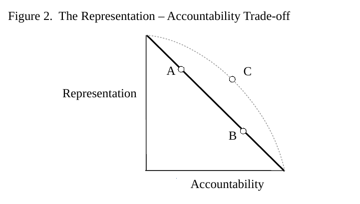
These arguments imply a trade-off between representation and accountability.  This is depicted in Figure 2.  Only if this trade-off takes the form of the bold diagonal line are we really prevented from rank-ordering electoral systems, however.  To see this, let A and B represent two hypothetical electoral systems.  Observe that A is as accountable as an electoral system could possibly be given its (high) level of representation, and that B is as representative as an electoral system could possibly be given its (high) level of accountability.  Trading A for B does not, therefore, result in a better electoral system; it merely changes the mixture of accountability and representation one gets.

Figure 2

Carey and Hix (2011) point out that the relationship between representation and accountability need not be unyielding; it could be curvilinear as indicated by the dashed line in Figure 2.  If so, there may exist an optimal electoral system, such as C.  Observe that if you were to replace C by another electoral system (i.e., any spot northwest or southeast of C on the dashed line), both representation and accountability would decline.  In this respect, C offers the best feasible mixture of representation and accountability.

PROBLEM 1:  MEASURING REPRESENTATION

Even were Carey and Hix’s optimistic view of the trade-off between representation and accountability to obtain, we would have to be able to measure representation and accountability accurately to identify an optimal electoral system.  This is not a trivial task.

Social choice theory considers how individual preferences combine to form collective choices.  A central result in social choice theory is that one cannot assume the transitivity of collective choices (Arrow 1951).  What does this mean?  Let’s say that three parties (A, B and C) contest a majority run-off election, and further that a majority of voters prefer A to B and B to C.  Social choice theory tells us that we cannot subsequently assume that there exists a majority for A over C; order the run-off differently or use a different electoral system (e.g., plurality rule or ranked ballots), and C could come out on top.[1]  This is a troubling result because it suggests that we cannot know whether an election result is representative – in the sense that it reflects the “will of the majority”  – or due merely to the vagaries of a particular electoral system.

Collective choices are almost certainly intransitive whenever voters evaluate more than two ballot options along several dimensions, such as when voters consider not only a party’s economic position but also its stance on regional autonomy or the charisma of its leader (McKelvey 1976).  In contrast, we can be reasonably sure that collective choices are transitive whenever voters have single-peaked preferences (Sen 1966).  This jargon implies that we can order voters in a single line such that all voters strictly prefer options (i.e., parties, candidates) that are closer to their position in the line to options further away.

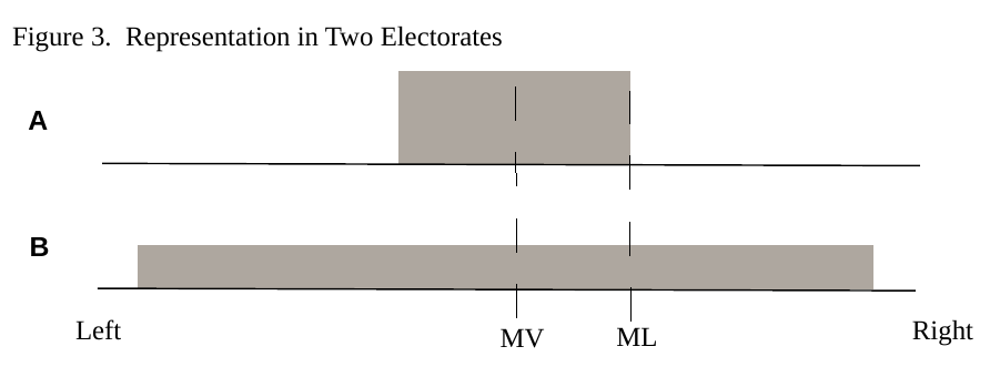
Whether or not voters have single-peaked preferences is an empirical question.  However, it is difficult to assess representation even when voters’ preferences are single-peaked.  Figure 3 depicts two stylized electorates, A and B.  The shaded blocks represent the ideological range of voters in each electorate.[2]  Thus, electorate A is moderate, with most voters just a bit to the left or right of the median voter (MV).  In contrast, electorate B is polarized, with many voters located far to the left or right of the median voter.  Elections place the median legislator (ML) as far away from the median voter in A as in B, and by that metric the electoral outcomes in A and B are equally representative.

Figure 3

The claim that the electoral outcomes in A and B are equally representative comes about because our measure of representation (congruence) ignores the variance in voters’ preferences.  A different view is that the electoral system in B has located the median legislator much closer to the median voter relative to the (wide) range of the electorate’s preferences than has the electoral system in AIndeed, the electoral system in A has located the median legislator at one extreme of voters’ preferences.  This reasoning suggests that we ought to evaluate congruence relative to the range of voters’ preferences.  Golder and Stramski (2011) do this, and find that judgments about the relative capacity of different electoral systems to deliver representative outcomes depends on how we measure representation. If we measure representation in terms of the simple distance between the median voter and median legislator, PR electoral systems outperform majoritarian systems. However, once we account for the range of voters’ preferences this difference disappears.

PROBLEM 2:  ELECTIONS MAY NOT DELIVER ACCOUNTABILITY

Electoral accountability is often seen to take the form of an implicit contract between voters and incumbents in which voters promise to re-elect incumbents only if their performance exceeds some standard (ill-defined or idiosyncratic as it may be).  Of course, voters would also prefer to elect better rather than worse candidates. Fearon (1999) argues that voters are unable to use elections to simultaneously motivate incumbents and select “good” candidates.

Fearon’s argument is based on a stylized 3-stage election cycle in which:

  1. An incumbent sets a policy, e.g., a target-level of unemployment. Voters want this policy to produce a particular outcome (e.g. zero unemployment), but they cannot precisely discern the degree to which the outcome is due to the incumbent’s policy or to other forces (e.g., world markets).
  1. After observing the policy outcome, voters either re-elect the incumbent or elect a replacement.
  1. The politician elected at Stage 2 sets another policy and the electoral cycle ends in a manner akin to the two-term limit that applies to American presidents.

At issue is how voters can cast their votes at Stage 2 to ensure that they get policy they want given three possible challenges.  The first challenge is to differentiate between “competent” politicians who can actually achieve the desired policy outcome and incompetent politicians who cannot.  The second challenge is to motivate politicians, all of whom prefer a different outcome than voters (perhaps because it’s hard work give voters what they want). The third challenge is a combination of the previous two, i.e., voters must both identify competent politicians and motivate reluctant incumbents.

Fearon shows that voters can meet the first two challenges by setting some standard, and re-electing the incumbent if achieve that standard.  For example, the voters say “We prefer zero unemployment, but if you deliver unemployment below 3 percent, we’ll re-elect you.”  This rule is sufficient to meet the first two challenges, that is, it allows voters to distinguish competent from incompetent incumbents in the first case, and to motivate reluctant politicians in the second case.

Surprisingly, however, this voting strategy fails in the third case.  The problem is that under such conditions voters cannot stick to their promise of re-electing an incumbent who achieves their standard.  To see this, observe that a re-elected incumbent will not work to deliver the policy that voters want at Stage 3 because the reward and motivation of re-election no longer apply. The voters’ choice is thus between an incumbent whom they know will ignore their policy preferences, on one hand, and a potentially competent challenger, on the other; voters always prefer the latter and so the incumbent might as well ignore the voters’ preferences at the outset.  With all incumbents, competent or not, behaving this way, the electorate cannot distinguish which are competent and which are not.[3] Elections thus fail to motivate incumbents or identify “good” candidates.

CONCLUSION

The fundamental problem in evaluating electoral systems in terms of these criteria is not necessarily that there exists an unyielding trade-off between representation and accountability. It is that we cannot reliably distinguish representative from unrepresentative electoral outcomes, either because these outcomes are products of a voting cycle or because our measures of representation are ambiguous.  The situation is no better with regard to accountability; even if we can state that the clarity of responsibility and the capacity to sanction incumbents is better under electoral system x than under electoral system y, there is no assurance that such conditions are sufficient to motivate or constrain office-holders.  It seems that we lack reliable means to connect electoral systems to two of the key guiding principles of representative government.  While this is a pessimistic conclusion, it should encourage citizens to carefully scrutinize politicians’ claims that some electoral systems are inherently “fairer”, “more democratic, “representative” or “effective” than others.

REFERENCES

Arrow, K. J. (1951). 1963. Social choice and individual values. Wiley, New York.

Carey, J. M., & Hix, S. (2011). The Electoral Sweet Spot: Low‐Magnitude Proportional Electoral Systems. American Journal of Political Science, 55(2), 383-397.

Downs, A. (1957). An Economic Theory of. Democracy, 599-608.

Duch, R. M., & Stevenson, R. T. (2008). The economic vote: How political and economic institutions condition election results. Cambridge University Press.

Fearon, J. D. (1999). Electoral accountability and the control of politicians: selecting good types versus sanctioning poor performance. Democracy, accountability, and representation, 55, 61.

Golder, M., & Stramski, J. (2010). Ideological congruence and electoral institutions. American Journal of Political Science, 54(1), 90-106.

Horowitz, Donald L. (2003). “Electoral Systems: A Primer for Decision Makers.” Journal of Democracy 14: 115-127.

McKelvey, R. D. (1976). Intransitivities in multidimensional voting models and some implications for agenda control. Journal of Economic theory, 12(3), 472-482.

Powell Jr, G. B., & Whitten, G. D. (1993). A cross-national analysis of economic voting: taking account of the political context. American Journal of Political Science, 391-414.

Powell, G. B. (2000). Elections as instruments of democracy: Majoritarian and proportional visions. Yale University Press.

Sen, A. K. (1966). A possibility theorem on majority decisions. Econometrica: Journal of the Econometric Society, 491-499.

[1]Formally, Arrow’s Theorem tells us that any electoral rule that respects certain minimal fairness criteria admits the possibility of an intransitive social choice.

[2]The fact that one can represent the preferences of voters in A and B as points along a straight line implies that they have single-peaked preferences.

[3]The reason that voters can stick to their promise in the first two scenarios is as follows.  Under the first scenario (i.e., when some politicians are competent and others not), voters can set a performance standard such that only competent incumbents are likely to be able to meet it.  And if the odds are that the incumbent is competent, the voters have every incentive to prefer them to a challenger who is as likely to be incompetent as not.

Under the second scenario, (i.e., all politicians are equally reluctant to carry out the voters’ preferred policy), voters know that any re-elected incumbent will do just as they please in their second term.  Thus, to properly motivate the politician in the first term, the voters must be able to credibly promise re-election given adequate performance in the first term.  Voters can stick to this promise because on all other grounds they are exactly indifferent between incumbents and challengers.  Given this indifference, it is clearly in the voters’ interest to maintain their re-election promise.


Is a non-partisan Senate a non-starter?

The final exam for my Strategy & Politics class always takes the same form:  I ask my students to apply what they have learned about game theory and parliamentary history to make sense of a contemporary political controversy.  The topic of this year’s exam was the partisan machinations around the Canadian Senate, that is, 1) the Conservatives’ threat to deploy their (temporary) Senate majority against the government’s legislative program, and 2) the Liberals’ promise to reform the Senate by installing non-partisan Senators via a “merit-based” selection process.  Will the Conservatives’ erect a Senate roadblock, and will the Liberals then break their promise and stack the Senate with Liberal hacks?  Or are both sides more likely to compromise, with the Conservatives passing duly diluted Liberal legislation through the Senate?

I always write up a template answer to the Strategy & Politics final exam that I give my students, and with the House’s attention now on Senate Reform, here’s my answer to my own question:

The Conservatives have threatened to use their Senate majority to stall the Liberals’ legislative program. (OK – they have toned down this kind of talk recently.) The Senate has the constitutional power to veto all legislation save that which is financial in nature. Furthermore, the Conservatives enjoy a majority in the Senate. To that extent the Conservatives’ threat is not an idle one. However, as Table 1 below shows, there are 22 vacancies in the Senate. Were Prime Minister Trudeau to fill these vacancies with loyal Liberals, the Conservative majority would vanish. But the Prime Minister has promised not to do this; instead, he proposes to appoint Senators on the basis of merit as recommended by a non-partisan board. Adding to the complexity of the situation is the fact that while in opposition Trudeau expelled Liberal Senators from the Liberal caucus. This implies that Liberal Senators are not bound by party discipline. Common ideological preferences may well lead many Liberal Senators to vote the party line, but it cannot be guaranteed.

Table 1. Party Standings in the Senate

Party N Seats
Conservative

45

Ind. Conservative

1

Ind. Liberal

28

Independent

9

Vacant

22

TOTAL

105

I consider 3 questions in light of this situation: 1) How can the Conservatives be expected to deploy their Senate majority? 2) How is the Government’s proposal likely to alter the situation? 3) Are the Liberals likely to follow through on their merit-based appointment process?

1. How can the Conservatives be expected to deploy their Senate majority?

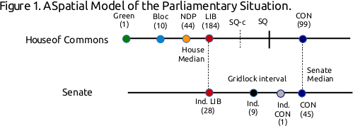
I use a a spatial model the parliamentary situation to understand how the Conservatives can be expected to deploy their Senate majority. Figure 1 depicts the distribution of parties along the left-right spectrum in both the House and the Senate. I assume that the parties are all perfectly cohesive (so a single ideal point suffices to represent the preferences of party members), and that parties’ respective positions are identical across the House and Senate. I also assume that the 9 independent Senators share an ideal point midway between the Liberals and the Conservatives; this will be a useful simplification. Actors have Euclidean preferences.

The Liberals enjoy a majority in the 338-seat House of Commons, and hence the median voter in the House is a Liberal MP; measures pass the House only with the support of this Liberal MP (i.e., the House median). Similarly, the median voter in the Senate is a Conservative; measures pass the Senate only with the support of this Senator (i.e., the Senate median). Policies in between the House and Senate medians cannot be moved. To appreciate this, consider the status quo policy, SQ, in this interval: if the Liberals try to replace SQ by an policy at their own ideal point, the Conservatives can use their Senate majority to veto the move; the policy will therefore remain at SQ.

Bicameral Game


The Conservatives cannot arbitrarily exercise their Senate veto. The Senate is an unelected body, and as such it lacks legitimacy among the Canadian electorate. To use it to veto every Liberal bill would allow the Liberals both to paint the Conservatives as obstructionist and to build a case to bypass the Senate (e.g., by abolition). I model this by assuming the Conservatives pay a cost, c > 0, for exercising their Senate veto. This cost creates an “envelope” of ±c around any status quo policy within which the Liberals have discretion. For example, were the Liberals to replace SQ by any point between SQ-c and SQ, the Conservative would allow it to pass because the cost of vetoing any such policy would exceed the gain associated with keeping policy at SQ.

The model highlights that the parliamentary situation is defined by a key relationship between two variables, the ideological distance between the Liberals and Conservatives, |LIB-CON|, and 2) c, the cost to the Conservatives for exercising their Senate veto. In particular, the Conservatives’ incentive to veto Liberal bills is strong only if they perceive the cost of deploying their veto to be small relative to the distance between their ideal point and the Liberals’, i.e., c << |LIB – CON|. Under opposite conditions, (i.e., c >> |LIB – CON|), the Conservatives would rarely have an incentive to use their Senate veto.

2. How is the Government’s proposal likely to alter the situation?

The reasoning above identifies conditions under which the Government’s proposal to appoint Senators on merit rather than partisanship is moot, i.e., c >> |LIB – CON|. The interesting case is one in which the Liberals’ and Conservatives’ positions are far apart, and Conservatives perceive the cost of a veto as quite small. Let’s assume that these more interesting conditions obtain.

Even so, how the Government’s proposed appointment process is likely to alter the parliamentary situation depends critically on the ideological distribution of meritorious individuals. Consider two reasonable possibilities: 1) that meritorious individuals are as likely to be left-wing as right-wing, or 2) that meritorious individuals are – in Canada, at least – likely to be left-of-centre in their ideology. These two situations are depicted in the top and bottom panels of Figure 2, respectively. The bell-curves in the panels reflect the (normal) ideological distribution of meritorious individuals, the set of people from which a putatively non-partisan board would select Senate appointees. For simplicity, the distance between the Liberals and Conservatives is scaled to be two standard deviations of this same ideological distribution.

Figure 2. Possible ideological distribution of meritorious individuals

What would be the effect of 22 non-partisan appointments were the ideological predisposition of those appointees as depicted in the top panel of Figure 2? Under such conditions one would expect approximately 3.5 appointees would hold positions to the Conservatives’ right.1 The Conservatives’ could expect the regular support of such individuals. Another 7.5 appointees could be expected to hold positions between the ideological centre (at 0) and the Conservatives’ position. The Conservatives would require the support of just 3 to 4 of these individuals to maintain a majority. The Senate median would therefore shift to the left under these conditions, but not by much; it would fall about midway between 0 and 1.2 Furthermore, the occasional defection of even 1 or 2 Liberal Senators (who, recall, are not under party discipline) would also dilute any leftward shift in the Senate median.

The bottom panel of Figure 2 depicts a situation where most meritorious individuals are to the left-of-centre. This is effected by shifting the ideological distribution of such people to the left by 1/2 standard deviations. As a consequence, the Conservatives could expect at most one of the 22 appointees to fall to their right, and only 5 such appointees would hold positions between 0 and 1. Thus at most 51 Senators (including the independent Conservative) would hold positions to the right of 0; the Senate median would thus fall just to the left of centre.

We are now in a position to answer the question set out above, that is, how will the Government’s proposed appointment process alter the parliamentary situation. The general answer is that it will shift the Senate median to the left – but by how much depends on the ideological distribution of meritorious individuals (and, to a lesser extent, on the cohesion of the Senate Liberals). If potential appointees are as likely to be right-wing as left-wing, the impact on the Senate median will be minimal; if most such individuals are left-wing, the Liberals’ appointment process may move the Senate median much closer to the Liberals’ position. However, the small number of Liberal Senators does put a limit on how much change the Liberals can effect in this way. Even if the ideological distribution of meritorious individuals were heavily right-skewed such that all 22 appointees were to the left of the Liberals, there would still only be 50 Senators at or to the left of the Liberal position, not enough to push the Senate median to the Liberals’ position. But the Liberals do not require that; to effect their agenda they simply require that the distance between the Senate median and their own position be less than c.

3. Are the Liberals likely to follow through on their merit-based appointment process?

The model establishes conditions under which one can expect the Liberals to break their promise to effect a truly non-partisan, merit-based appointment process.

  • c |LIB-CON|: it is costless for the Liberals to keep their promise because they can effect their legislative agenda regardless of the Conservatives’ Senate majority. Under these conditions, the Liberal proposal for Senate appointments is mere window-dressing.
  • c < |LIB-CON| and the ideological distribution of meritorious individuals is symmetric: The Liberals are likely to break their promise under these conditions. This is is because a non-partisan, merit-based appointment process will leave the Senate median close to the Conservatives’ position, allowing the Conservatives to block much of the Liberal agenda. The smaller c is relative to the ideological distance between the two parties, the stronger the incentive for the Liberals to stack the Senate, either overtly or covertly by politicizing the “non-partisan” appointment process.
  • c < |LIB-CON| and the ideological distribution of meritorious individuals is right-skewed: The situation is unpredictable. On one hand, by simply keeping their promise, the Liberals would be able to effect a significant leftward shift in the Senate median. If the resulting distance between the Senate median and the Liberals’ position was then less than c, one could expect the Liberals to keep their promise because even a non-partisan appointment process would enable them to effect their legislative agenda. However, were the resulting distance between the Senate median and the Liberals’ position to still be greater than c, the Liberals would likely break their their promise and stack the Senate provided they felt that they could count on the unwavering support of both sitting Liberal Senators and their “non-partisan” appointees.

1Given 22 appointees and a .16 probability that an appointee would hold a position at or to the Conservatives’ right, one would expect 3.5 appointees to hold positions at or to the Conservatives’ right.

2In fact, one can use the normal distribution to compute that the Senate median would fall at .45 standard deviations to the right of 0.

Votes & Seats under the Alternative Vote

In this post, I consider the proportionality of the Alternative Vote (AV), that is, the degree to which AV produces a 1:1 ratio between parties’ vote shares and their seat shares. (AV is the electoral system that is purportedly the Liberal’s favoured alternative to replace Canada’s first-past-the-post electoral system (FPTP).)

By using data from Australian federal elections as well as state elections in Australia’s five mainland states, we can see how AV tends to perform in six different polities.* Moreover, because these jurisdictions all employed FPTP at some point in time, we can also consider whether the shift to AV altered the votes-seats proportionality of Australian elections. This should give us some idea of what to expect should Canada adopt AV.

A priori, we should not expect AV to be any more or less proportional than FPTP. The reason is that both system tend to employ single-member districts. The number of seats per district—what political scientists call the district magnitude—constrains the proportionality of an electoral system quite independently of the formula that is used to translate votes into seats. The higher the district magnitude, the more closely the division of seats among parties can approximate the distribution of vote shares among parties. This improves the votes-seats proportionality of the electoral system. Conversely, votes-seats proportionality that is achievable declines as the district magnitude moves to 1.

Understand that the impact of district magnitude on votes-seats proportionality operates at the district-level. It’s quite possible for an electoral system based on single-member districts to be proportional in aggregate even as it is highly disproportional in every district. Imagine a polity with three parties (A, B, C) competing in FPTP elections in three single-member districts (1,2 3). Assume that party A wins 34% of the vote in district 1 versus 33% for parties B and C, respectively. Similarly, B wins district 2, and C wins district 3, on identical divisions of the vote, that is, 34% – 33% – 33%. The result is a high degree of disproportionality within each district (the party winning 34% of the vote obtaining 100% of the district’s seats) but perfect proportionality in the aggregate, each party winning 1/3 of the seats on 1/3 of the vote.

Of course, district-level disproportionality need not (and often does not) cancel out across districts; it may well be compounded. Indeed, in the past governing parties would intentionally gerrymander and malapportion districts to ensure that disproportionality compounded across districts: district boundaries were drawn to ensure that the government won the vast majority of seats by razor-thin margins whilst the opposition’s votes were concentrated in a few districts which it would win by massive margins. But disproportionality can also be compounded across districts because of how voters cast their votes. In closely contested multi-party elections supporters of 3rd place parties tend to defect to one of the two leading parties in their district. In the aggregate this results in the top-two vote-winning parties obtaining seat shares in excess of their votes and 3rd+ place parties obtaining seat shares below their vote shares.

Votes & Seats in Canada under FPTP

Figure 1. (right-click to enlarge)

This pattern is visible in Figure 1, which shows the relationship between vote- and seat-shares at Canadian general elections since 1949. A perfectly proportional electoral system would allocate seat shares to parties such that all outcomes fell on the dashed 45° line, indicating a 1:1 ratio between parties’ vote-shares and seat-shares. Instead, what we see is that the red and blue dots (representing the Liberals and Conservatives, respectively) are consistently above the 45° line whenever their vote-shares exceed 35 percent. Correspondingly (because elections are zero-sum), parties with vote-shares below 35% consistently fall below the 45° line. The few exceptions to this rule are regional parties (notably the Bloc Quebecois and Reform).

We can describe the Canadian data more precisely by regressing parties’ seat-shares (S%it) on their vote-shares (V%it) and a set of election-year fixed effects (Yt):

S%it = a + bV%it + dYt + uit [1]

Disproportionality is signalled by b 1. Estimating Eq. 1 via OLS yields

b = 1.28 (.03)

Adj. R2 = .88  RMSE = 7.20

N Obs = 119  N Clusters = 22

Huber-White SE clustered by election in parentheses

No surprise here: Canada’s FPTP electoral system is quite disproportional.

It is interesting and informative to modify Eq. 1 to include the square of parties’ vote shares.

S%it = a + b1V%it + b2V2%it + dYt + uit [1b]

This specification allows for nonlinear and increasing returns to votes. Estimating Eq. 1b via OLS yields:

b1 = .06 (.11)  b2 = .028 (.002)

Adj. R2 = .95  RMSE = 4.74

N Obs = 119  N Clusters = 22

Huber-White SE clustered by election in parentheses

These results tell us that the marginal effect of votes on seats in Canada increases as the party’s vote-share increases. To be precise, a party’s seat-share increases by .06 + .028V%it for every 1% of the vote the party wins. So the larger a party’s vote-share, the greater the rate at which it translates votes into seats. In fact, one can deduce that the Canadian system’s “break-even” point is 33.6% of the vote; every 1 percent of the vote won after this point returns greater than 1 percent of seats.

Votes & Seats in Australia

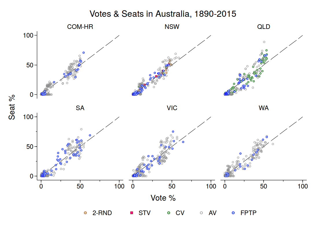
The Canadian data provide a context within which to consider the proportionality of Australia’s AV electoral system. Figure 2 below shows vote shares and seat shares at Australian federal and state elections since 1890. The colour coding in Figure 2 varies by electoral system. So one sees the relationship between votes and seats under not just FPTP and AV but also the Contingent Vote (CV) in Queensland, and STV and 2-round plurality in NSW.

Figure 2. (right-click to enlarge)

Oz Votes and Seats

I find three things noteworthy about Figure 2.

  1. Australian elections are characterized by disproportionality. Observe that parties that obtain 35-40+% of the vote tend to have seat-shares that fall above the 45° line that marks perfect proportionality.
  2. Disproportionality at Australian elections does not appear as severe as it is at Canadian elections. It’s really only in Queensland that the return to votes is visibly non-linear and increasing.
  3. It’s not obvious on these data that elections under FPTP were significantly more disproportional than those held under AV.

Of course, these are just my impressions of the visual data; it’s worth exploring the data more systematically. Now, in assessing the votes-seats proportionality of Australian elections we want to:

  • account for the fact that some of these elections employed multi-member districts;
  • allow the relationship between votes and seats to vary by state; and
  • identify the impact on proportionality of shifting from FPTP to AV.

I do all this by: i) controlling for the average district magnitude at election t in state j (Mtj); ii) adding state fixed-effects (STATEj) to the model and interacting these state fixed-effects with parties’ vote-shares (V%ijt); and iii) including a dummy variable, AVjt , that equals 1 when AV is used and 0 when FPTP is used. (Elections that employed other electoral systems are dropped.) The model is

S%iit = a + d1Mtj + d2Yt + d3STATEj + b1V%ijt + b2(V%ijt * STATEj) [2]

+ b3(V%ijt * AVjt) + b4(V%ijt * STATEj * AVjt) + eijt.

The quantity of interest here remains the marginal effect of votes on seats, that is, the rate at which vote-shares are translated into seat-shares. The interactions between V%ijt and STATEj and AVjt in Eq 2 allow this rate to vary by state and by electoral system.

Figure 3. (right-click to enlarge)

Figure 3 shows the marginal effect of votes on seats for each state under FPTP and AV. The circles represent the point estimates, and the bars show the 90% confidence intervals surrounding these estimates. So what Figure 3 tells us, for example, is that for every 1% of the vote a party won at elections to the Commonwealth’s House of Representatives (COM-HR) it obtained about 1.08% of the assembly’s seats on average. In other words, Australian federal elections are mildly disproportional. Furthermore, the proximity of the blue and gray dots tells us that the relationship between votes and seats at Commonwealth elections was unaffected by the shift from FPTP to AV.

In the main, the same remarks can be extended to all five mainland states. Only Victorian elections – held under FPTP no less – might, maybe have been proportional. In no state did AV make elections reliably more proportional – though it came close to doing so in Western Australia. Of course, Australian elections were never as disproportional as Canadian federal elections; only elections in Queensland come close – and that probably has a lot more to do with how the Nicklin and Bjelke-Petersen governments malapportioned and gerrymandered electoral districts than the electoral system itself.

To better isolate any causal effect of the electoral system on votes-seats disproportionality, I estimated Eq. 2 again, but with the data limited to just the very last elections held under FPTP and the elections held immediately thereafter on the adoption of AV. This eliminated NSW from the analysis (because NSW experimented with several electoral systems between abandoning FPTP and adopting AV). District magnitudes did not vary within states at these transitional elections, so there was also no need to control for the average district magnitude. The model was then:

S%iit = a + d1STATEj + b1V%ijt + b2(V%ijt * AVjt) + eijt [2b]

Under this model, the marginal effect of vote-shares on seat-shares under FPTP is given by b1, whilst under AV it’s given by b1 + b2. Estimating Eq. 2 via OLS returned 

b1 = 1.10 (.04)  b2 = -.04 (.08)

Adj. R2 = .88  RMSE = 8.51

N Obs = 47  N Clusters = 10

Huber-White SE clustered by election in parentheses

Thus the ratio of vote- to seat-shares was 1:1.10 under FPTP and declined to 1:1.06 under AV – BUT this decline is not statistically significant (not by a long-shot). In other words, we can’t rule out that the shift to AV made no difference whatsoever.

Finally, I estimated an Australian analogue to Eq 1b. containing parties’ vote shares and their squared vote shares – but only using data from AV elections:

S%iit = a + d1Yt + d2STATEj + b1V%ijt b2V2%ijt + eijt [3]

Estimating Eq. 3 via OLS yields:

b1 = .89 (.06)  b2 = .004 (.0016)

Adj. R2 = .88  RMSE = 6.56

N Obs = 1209  N Clusters = 180

Huber-White SE clustered by election in parentheses

These results indicate that AV also generates nonlinear and increasing returns to votes, although not nearly so sharply as in Canada.  The “break-even” point under AV is also lower at 27.5%

Discussion

There’s no reason to expect AV to be any more proportional an electoral system than FPTP. This is because the proportionality of the electoral system is tightly constrained by the number of seats per district, and both AV and FPTP are typically used with single-member districts.

The data from Australian state and federal elections are consistent with this theoretical expectation. Australian elections do not produce the level of disproportionality that is observed in Canadian elections – but this probably has little to do with Australia’s AV electoral system because the adoption of AV in favour of FPTP in Australia had no discernible impact on electoral disproportionality.

What does this mean for electoral reform in Canada? These data suggest that we should not expect the disproportionality of the Canadian electoral system to change appreciably were the Government to choose AV to replace FPTP. Disproportionality systematically favours larger parties over smaller parties, and to that extent the Conservatives should not be particularly apprehensive of a transition to AV. As I observed previously, a shift to AV could position the Conservatives as a right-wing version of the ALP – not often in government, but dominant on their part of the political spectrum. Correspondingly, the NDP and the Greens should not expect an AV electoral system on its own to improve the efficiency with which these two parties translate votes into seats.

In my next post I’ll explore another aspect of AV – it’s volatility.


* A big thanks to my colleague, Campbell Sharman for furnishing me with these data.