R studio/ leaflect | A CHERRY CHEN PORTFOLIO

Vancouver crime data project with R – write up

Process:

With the original crime data that obtained from the course website, that is the Vancouver crime data over the past decade and even further. My focus was only the crime data from 2013, so the first step is to extract those 2013 data out of the original data.

After give it a nice title and date and description, it is time to start the processing script in R studio. The first step is to acquire data from where I stored it, and I ran the program to allow R read the data in. After get data into R, the next step is to parse the data that I organized the data into a nicer format such as changing addresses into an accurate format and finding longitudes and latitudes for each address. The next step is data mining, and that is to examine those large pre-existing data in order to generate new information. In this step, I have grouped different kinds of crimes together just to make the data set more clear and easy to understand when they turn out on an interactive web map. After the mining step is the filtering step, and this step is simply to get rip of the data that are not located within city of Vancouver. After organizing these data, they need to be converted into shapefiles so they can actually appear on a web map. After that, I aggregate the data to a grid so those data will appear on correct location.

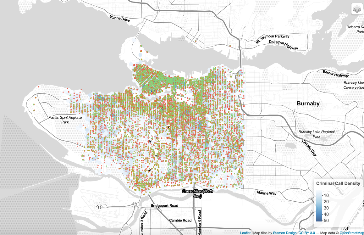
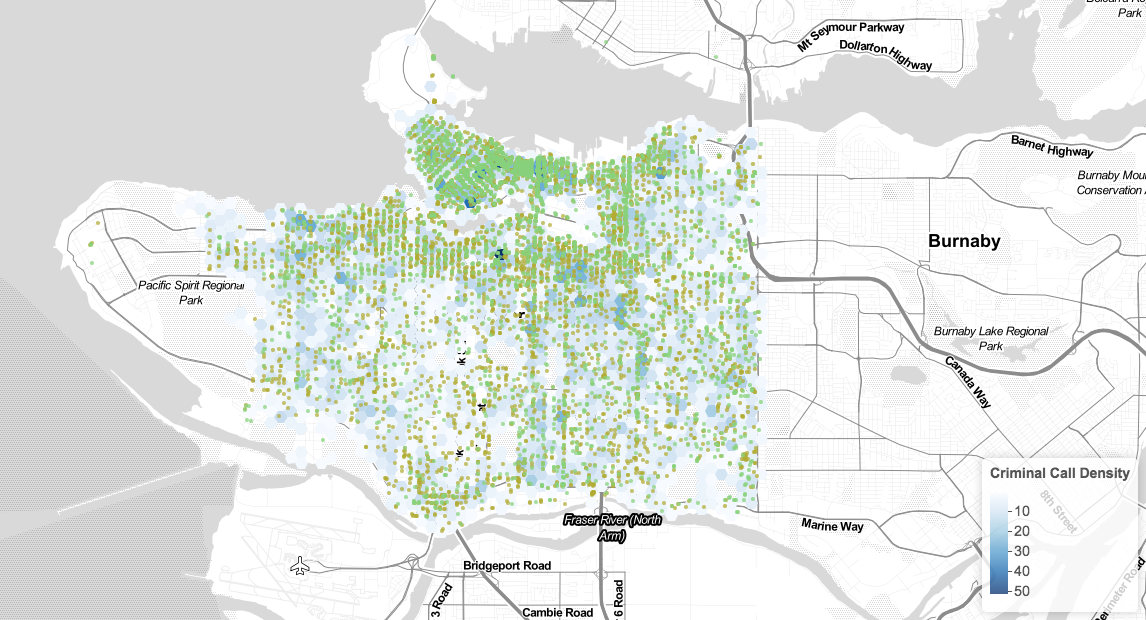
When have all the data prepared and organized, now is time to make the map! I have four groups of crime types, and I have assigned them different cids, and that is just for the ease of later use of program running. In order to add those points onto the map, I have added “circle markers” and have assigned different types of crime different colors, and I add the Vancouver map (work like the base map) onto it. Now is to add the layer control panel so that the map can be an interactive one! After that is time to add those hex polygons onto the map along with the points that I just added, and those polygons shows the frequency of total crime calls. Now the map is almost done, by putting the toggleable layer and point layer together and an interactive map is generated.

I started with 34,355 records from the 2013 crime data and end up with 30,390 records after organized.

There are some errors but definitely not a lot, as we can still see some data that are not being filtered out, but most of the data are looking good. So I would say the data is quite reliable.

Shape file: a shape file stores geographic features such as points, lines, or polygons onto a base map.

Csv file: a csv file is used to store tabular data and make it into a database.

Excel: it is a spreadsheet and widely used software and it can be saved as a csv file.

Geojson: it is used to representing simple geographical features. Json stands for JavaScript Object Notation.

Visualization:

By using R, I realized that this is a powerful program as it basically makes maps by coding. For cartographic design, I think that is hard to adjust the colors, as I am not familiar with this software. I may have lots of ideas in mind, but I am not sure how to apply into R, so I can only change the colors of the hex polygon and the points that shown on the map. I cannot write a full script by myself, so I can only use what I have, and that is being say, I cannot really design my own map.

The hex polygon looks very gentle as it is used to show the frequency, as I saw from the map, Vancouver’s west side has a lower frequency of crimes and Vancouver East and downtown area have a higher frequency. Crime types vary from area to area, for example, downtown has a higher rate of “break into commercial.” There are other data that may be useful in this data such as assaults and robs.

Reflection:

In my opinion, proprietary software is more secure as users pay to buy it, and if users have any problem, there must be a way to solve it. But the downside of proprietary software is that users cannot write their own codes, before purchasing it, users have to read through los of policy and sign agreements while open source software allows users to write and generate their own codes, which give more freedom to users who prefer to do so. I used to use Adobe Illustrator to make maps, by using R for this project, I realized that R is a really powerful tool to do lots of things, and one of the strength of R is once we have the codes, we can rewrite a map or generate a new map as many time as we want as long as we have the codes; while in Adobe Illustrator, each time we want to start a new map, we need to make it from scratch.

[code: language=”R”]

######################################################

# Vancouver crime 2013: Data Processing Script

# Date: 10/24

# By: Cherry Chen

# Desc: An interactive map showing City of Vancouver crime events in 2013

######################################################

# —————————————————————— #

# —————————- Acquire —————————– #

# —————————————————————— #

# access from the interwebz using “curl”

fname = “/Users/Acherry/Desktop/crime_2013.csv”

geo_csv = “/Users/Acherry/Desktop/crime_2013_geocoded.csv”

# Read data as csv

data = read.csv(fname, header=T)

# inspect your data

print(head(data))

# ————————————————- #

# ————– Parse: Geocoder ——————- #

# ————————————————- #

# change intersection to 00’s

data$h_block = gsub(“X”, “0”, data$HUNDRED_BLOCK)

print(head(data$h_block))

# Join the strings from each column together & add “Vancouver, BC”:

data$full_address = paste(data$h_block,“Vancouver, BC”,

sep=“, “)

# a function taking a full address string, formatting it, and making

# a call to the BC government’s geocoding API

bc_geocode = function(search){

# return a warning message if input is not a character string

if(!is.character(search)){stop(“‘search’ must be a character string”)}

# formatting characters that need to be escaped in the URL, ie:

# substituting spaces ‘ ‘ for ‘%20’.

search = RCurl::curlEscape(search)

# first portion of the API call URL

base_url = “http://apps.gov.bc.ca/pub/geocoder/addresses.json?addressString=”

# constant end of the API call URL

url_tail = “&locationDescriptor=any&maxResults=1&interpolation=adaptive&echo=true&setBack=0&outputSRS=4326&minScore=1&provinceCode=BC”

# combining the URL segments into one string

final_url = paste0(base_url, search, url_tail)

# making the call to the geocoding API by getting the response from the URL

response = RCurl::getURL(final_url)

# parsing the JSON response into an R list

response_parsed = RJSONIO::fromJSON(response)

# if there are coordinates in the response, assign them to `geocoords`

if(length(response_parsed$features[[1]]$geometry[[3]]) > 0){

geocoords = list(lon = response_parsed$features[[1]]$geometry[[3]][1],

lat = response_parsed$features[[1]]$geometry[[3]][2])

}else{

geocoords = NA

}

# returns the `geocoords` object

return(geocoords)

}

# Geocode the events – we use the BC Government’s geocoding API

# Create an empty vector for lat and lon coordinates

lat = c()

lon = c()

# loop through the addresses

for(i in 1:length(data$full_address)){

# store the address at index “i” as a character

address = data$full_address[i]

# append the latitude of the geocoded address to the lat vector

lat = c(lat, bc_geocode(address)$lat)

# append the longitude of the geocoded address to the lon vector

lon = c(lon, bc_geocode(address)$lon)

# at each iteration through the loop, print the coordinates – takes about 20 min.

print(paste(“#”, i, “, “, lat[i], lon[i], sep = “,”))

}

# add the lat lon coordinates to the dataframe

data$lat = lat

data$lon = lon

# after geocoding, it’s a good idea to write your file out!

# you will need to modify the directory where you want R to write

# your data!

ofile = “/Users/Acherry/Desktop/crime_2013_geocoded.csv”

write.csv(data, ofile)

# read in geocoded data

geo_csv = “/Users/Acherry/Desktop/crime_2013_geocoded.csv”

data = read.csv(geo_csv, header = T)

# ————————————————- #

# ——————— Mine ———————- #

# ————————————————- #

# — Examine the unique cases — #

# examine how the cases are grouped – are these intuitive?

unique(data$full_address)

unique(data$NEIGHBOURHOOD)

# examine the types of cases – can we make new groups that are more useful?

# Print each unique case on a new line for easier inspection

for (i in 1:length(unique(data$TYPE))){print(unique(data$TYPE)[i], max.levels=0)}

# — theft —#

# Theft_from_Vehicle

# Other_Theft

# Theft_of_Vehicle

# — break and enter —#

#Break and Enter Residential / Other

#Break and Enter Commercial

# — Offence and mischief —#

#Offence Against a Person

#Mischief

# — homicide —#

#Homicide

#————————————————————–#

#——————–Groupping———————————#

#————————————————————–#

# theft

theft = c(‘Theft from Vehicle’,’Other Theft’,’Theft of Vehicle’)

# break and enter

break_enter = c(‘Break and Enter Residential/Other’,’Break and Enter Commercial’)

# offence and mischief

Offence_mischief = c(‘Offence Against a Person’,’Mischief’)

# homicide

homicide = c(‘Homicide’)

#——–give class id numbers:—————–#

data$cid = 9999

for(i in 1:length(data$TYPE)){

if(data$TYPE[i] %in% theft){

data$cid[i] = 1

}else if(data$TYPE[i] %in% break_enter){

data$cid[i] = 2

}else if(data$TYPE[i] %in% Offence_mischief){

data$cid[i] = 3

}else if(data$TYPE[i] %in% homicide){

data$cid[i] = 4

}

———————————————————————

# — handle overlapping points — #

# Set offset for points in same location:

data$lat_offset = data$lat

data$lon_offset = data$lon

# Run loop – if value overlaps, offset it by a random number

for(i in 1:length(data$lat)){

if ( (data$lat_offset[i] %in% data$lat_offset) && (data$lon_offset[i] %in% data$lon_offset)){

data$lat_offset[i] = data$lat_offset[i] + runif(1, 0.0001, 0.0005)

data$lon_offset[i] = data$lon_offset[i] + runif(1, 0.0001, 0.0005)

}

# —————————————————————— #

# —————————- Filter —————————— #

# —————————————————————— #

# Subset only the data if the coordinates are within our bounds or if

# it is not a NA

data_filter = subset(data, (lat <= 49.313162) & (lat >= 49.199554) &

(lon <= -123.019028) & (lon >= -123.271371) & is.na(lon) == FALSE )

# plot the data

plot(data$lon, data$lat)

plot(data_filter$lon, data_filter$lat)

# If everthing looks good, we might also write out our file:

ofile_filtered = ‘/Users/Acherry/Desktop/crime_2013_filtered.csv’

write.csv(data_filter, ofile_filtered)

# — Convert Data to Shapefile — #

# store coordinates in dataframe

crime_2013 = data.frame(data_filter$lon_offset, data_filter$lat_offset)

# create spatialPointsDataFrame

data_shp = SpatialPointsDataFrame(coords = crime_2013, data = data_filter)

# set the projection to wgs84

projection_wgs84 = CRS(“+proj=longlat +datum=WGS84”)

proj4string(data_shp) = projection_wgs84

# set an output folder for our geojson files:

geofolder = “/Users/Acherry/Desktop/crime_2013_geocoded.csv”

# Join the folderpath to each file name:

opoints_shp = paste(geofolder, “calls_”, “1401”, “.shp”, sep = “”)

print(opoints_shp) # print this out to see where your file will go & what it will be called

opoints_geojson = paste(geofolder, “calls_”, “1401”, “.geojson”, sep = “”)

print(opoints_geojson) # print this out to see where your file will go & what it will be called

# write the file to a shp

writeOGR(data_shp, opoints_shp, layer = “data_shp”, driver = “ESRI Shapefile”,

check_exists = FALSE)

# write file to geojson

writeOGR(data_shp, opoints_geojson, layer = “data_shp”, driver = “GeoJSON”,

check_exists = FALSE)

# — aggregate to a grid — #

# ref: http://www.inside-r.org/packages/cran/GISTools/docs/poly.counts

# set the file name – combine the shpfolder with the name of the grid

grid_fn = ‘https://raw.githubusercontent.com/joeyklee/aloha-r/master/data/calls_2014/geo/hgrid_250m.geojson’

# read in the hex grid setting the projection to utm10n

hexgrid = readOGR(grid_fn, ‘OGRGeoJSON’)

# transform the projection to wgs84 to match the point file and store

# it to a new variable (see variable: projection_wgs84)

hexgrid_wgs84 = spTransform(hexgrid, projection_wgs84)

# Use the poly.counts() function to count the number of occurrences of calls per grid cell

grid_cnt = poly.counts(data_shp, hexgrid_wgs84)

# define the output names:

ohex_shp = paste(geofolder, “hexgrid_250m_”, “1401”, “_cnts”,

“.shp”, sep = “”)

print(ohex_shp)

ohex_geojson = paste(geofolder, “hexgrid_250m_”,”1401″,”_cnts”,”.geojson”)

print(ohex_geojson)

# write the file to a shp

writeOGR(check_exists = FALSE, hexgrid_wgs84, ohex_shp,

layer = “hexgrid_wgs84”, driver = “ESRI Shapefile”)

# write file to geojson

writeOGR(check_exists = FALSE, hexgrid_wgs84, ohex_geojson,

layer = “hexgrid_wgs84”, driver = “GeoJSON”)

#———————————————#

#—————–LEAFLET———————#

#———————————————#

# install the leaflet library

install.packages(“leaflet”)

# add the leaflet library to your script

library(leaflet)

# initiate the leaflet instance and store it to a variable

m = leaflet()

# we want to add map tiles so we use the addTiles() function – the default is openstreetmap

m = addTiles(m)

# we can add markers by using the addMarkers() function

m = addMarkers(m, lng=-123.256168, lat=49.266063, popup=”T”)

# we can “run”/compile the map, by running the printing it

#below READ DATA BK

filename = “/Users/Acherry/Desktop/crime_2013_filtered.csv”

# data_filter = read.csv(“/Users/Acherry/Desktop/crime_2013_filtered.csv”, header = TRUE)

# subset out your data_filter:

df_theft = subset(data_filter, cid == 1)

df_break_enter = subset(data_filter, cid == 2)

df_Offence_mischief = subset(data_filter, cid == 3)

df_homicide = subset(data_filter, cid == 4)

# initiate leaflet

m = leaflet()

# add openstreetmap tiles (default)

m = addTiles(m)

# you can now see that our maptiles are rendered

colorFactors = colorFactor(c(‘#E65946’, ‘#5CE646’, ‘#DA6526’, ‘#88D27C’),

domain = data_filter$cid)

m = addCircleMarkers(m,

lng = df_theft$lon_offset, # we feed the longitude coordinates

lat = df_theft$lat_offset,

popup = df_theft$TYPE,

radius = 2,

stroke = FALSE,

fillOpacity = 0.75,

color = colorFactors(df_theft$cid),

group = “1 – theft”)

m = addCircleMarkers(m,

lng = df_break_enter$lon_offset, lat=df_break_enter$lat_offset,

popup = df_break_enter$TYPE,

radius = 2,

stroke = FALSE, fillOpacity = 0.75,

color = colorFactors(df_break_enter$cid),

group = “2 – break and enter”)

m = addCircleMarkers(m,

lng = df_Offence_mischief$lon_offset, lat=df_Offence_mischief$lat_offset,

popup = df_Offence_mischief$TYPE,

radius = 2,

stroke = FALSE, fillOpacity = 0.75,

color = colorFactors(df_Offence_mischief$cid),

group = “3 – Offence and mischief”)

m = addCircleMarkers(m,

lng = df_homicide$lon_offset, lat=df_homicide$lat_offset,

popup = df_homicide$TYPE,

radius = 2,

stroke = FALSE, fillOpacity = 0.75,

color = colorFactors(df_homicide$cid),

group = “4 – homicide”)

m = addTiles(m, group = “OSM (default)”)

m = addProviderTiles(m,”Stamen.Toner”, group = “Toner”)

m = addProviderTiles(m, “Stamen.TonerLite”, group = “Toner Lite”)

m = addLayersControl(m,

baseGroups = c(“Toner”,”Toner Lite”),

overlayGroups = c(“1 – theft”, “2 – break_enter”,

“3 – Offence_mischief”,”4 – homicide”))

# make the map

—————————————————————————–

# subset out your data_filter:

df_theft = subset(data_filter, cid == 1)

df_break_enter = subset(data_filter, cid == 2)

df_Offence_mischief = subset(data_filter, cid == 3)

df_homicide = subset(data_filter, cid == 4)

# Now we’re going to put those variables into a **list** so we can loop through them:

data_filterlist = list(df_theft = subset(data_filter, cid == 1),

df_break_enter = subset(data_filter, cid == 2),

df_Offence_mischief = subset(data_filter, cid == 3),

df_homicide = subset(data_filter, cid == 4))

# Remember we also had these groups associated with each variable? Let’s put them in a list too:

layerlist = c(“1 – theft”,”2 – break_enter”,”3 – Offence_mischief”,”4 – homicide”)

# We can keep that same color variable:

colorFactors = colorFactor(c(‘#E65946’, ‘#5CE646’, ‘#DA6526’, ‘#88D27C’), domain=data_filter$cid)

# Now we have our loop – each time through the loop, it is adding our markers to the map object:

for (i in 1:length(data_filterlist)){

m = addCircleMarkers(m,

lng=data_filterlist[[i]]$lon_offset,

lat=data_filterlist[[i]]$lat_offset,

popup=data_filterlist[[i]]$TYPE,

radius=2,

stroke = FALSE,

fillOpacity = 0.75,

color = colorFactors(data_filterlist[[i]]$cid),

group = layerlist[i]

)}

m = addTiles(m, “Stamen.TonerLite”, group = “Toner Lite”)

m = addLayersControl(m,

overlayGroups = c(“Toner Lite”),

baseGroups = layerlist

)

——————–polygon—————————————————–

# define the filepath

hex_1401_fn = ‘https://raw.githubusercontent.com/joeyklee/aloha-r/master/data/calls_2014/geo/hgrid_250m_1401_counts.geojson’

# read in the geojson

hex_1401 = readOGR(hex_1401_fn, “OGRGeoJSON”)

m = leaflet()

m = addProviderTiles(m, “Stamen.TonerLite”, group = “Toner Lite”)

# Create a continuous palette function

pal = colorNumeric(

palette = “Blues”,

domain = hex_1401$data

)

# add the polygons to the map

m = addPolygons(m,

data = hex_1401,

stroke = FALSE,

smoothFactor = 0.2,

fillOpacity = 1,

color = ~pal(hex_1401$data),

popup = paste(“Number of crimes: “, hex_1401$data, sep=“”)

)

m = addLegend(m, “bottomright”, pal = pal, values = hex_1401$data,

title = “Criminal Call Density”,

labFormat = labelFormat(prefix = ” “),

opacity = 0.75

)

————————————synthesis———————————————

# initiate leaflet map layer

m = leaflet()

m = addProviderTiles(m, “Stamen.TonerLite”, group = “Toner Lite”)

# — hex grid — #

# store the file name of the geojson hex grid

hex_1401_fn = ‘https://raw.githubusercontent.com/joeyklee/aloha-r/master/data/calls_2014/geo/hgrid_250m_1401_counts.geojson’

# read in the data

hex_1401 = readOGR(hex_1401_fn, “OGRGeoJSON”)

# Create a continuous palette function

pal = colorNumeric(

palette = “Blues”,

domain = hex_1401$data

)

# add hex grid

m = addPolygons(m,

data = hex_1401,

stroke = FALSE,

smoothFactor = 0.2,

fillOpacity = 1,

color = ~pal(hex_1401$data),

popup= paste(“Number of crimes: “,hex_1401$data, sep=“”),

group = “hex”

)

# add legend

m = addLegend(m, “bottomright”, pal = pal, values = hex_1401$data,

title = “Criminal Call Density”,

labFormat = labelFormat(prefix = ” “),

opacity = 0.75

)

# — points data — #

# subset out your data:

df_theft = subset(data_filter, cid == 1)

df_break_enter = subset(data_filter, cid == 2)

df_Offence_mischief = subset(data_filter, cid == 3)

df_homicide = subset(data_filter, cid == 4)

data_filterlist = list(df_theft = subset(data_filter, cid == 1),

df_break_enter = subset(data_filter, cid == 2),

df_Offence_mischief = subset(data_filter, cid == 3),

df_homicide = subset(data_filter, cid == 4))

layerlist = c(“1 – theft”, “2 – break_enter”,

“3 – Offence_mischief”,“4 – homicide”)

colorFactors = colorFactor(c(‘#E65946’, ‘#5CE646’, ‘#DA6526’, ‘#88D27C’), domain=data_filter$cid)

for (i in 1:length(data_filterlist)){

m = addCircleMarkers(m,

lng=data_filterlist[[i]]$lon_offset, lat=data_filterlist[[i]]$lat_offset,

popup=data_filterlist[[i]]$TYPE,

radius=2,

stroke = FALSE, fillOpacity = 0.75,

color = colorFactors(data_filterlist[[i]]$cid),

group = layerlist[i]

)

}

m = addLayersControl(m,

overlayGroups = c(“Toner Lite”, “hex”),

baseGroups = layerlist

)

# show map

[ /code]