Final Project

My final project was on Lyme Disease, conducted with a group of 3 of my classmates: Alexander Coster, Chelsey Cu and Lakshmi Soundarapandian.

We looked at historic and current distributions on lyme disease cases in the northeastern United States and used the data to extrapolate future distributions of lyme disease in view of climate change. We tested 3 models using maxent to determine which variables are the most important in determining tick habitat and survival, from which we inferred lyme disease distribution. We then used the most significant variables to construct a range of future distribution using predicted environmental and biological data. A more in depth description of our study can be accessed on the project blog here or a brief powerpoint of the study is available here.

Comparative Modelling Approaches for Understanding Urban Violence – Review

The main purpose of the paper is to provide a greater understanding of the factors that influence heterogeneous distributions of crime. The authors focus on the comparative analysis of three quantitative approaches: Ordinary Least Squares (OLS), Geographically Weighted Regression (GWR) and Data Envelopment Analysis (DEA). The above methods are then applied to explore the structural theories of violence in Cincinnati, Ohio by block group. To predict assault rates between January and June of 2008 the authors use 2006 population density from Caliper Corporation, density of alcohol outlets from the Ohio Division of Liquor Control, and social disorganization calculated from socio-economic disadvantage, female headed-households, and residential instability, as independent variables.

The presentation can be accessed here and the more detailed review can be accessed here.

Bibliography

Grubesic, T. H., Mack, E. A., Kaylen, M. T. (2012). Comparative modeling approaches for understanding urban violence. Social Science Research, 41(1), 92-109.doi:10.1016 /j.ssresearch.2011.07.004

Use of GIS by fire departments

For me this was one of the most interesting and exciting lectures as we got to see in great detail crucial real-world GIS applications. This lecture used the example of the Calgary Fire Department and their use of GIS in planning for the future, deciding where to locate new stations and apparatus deployment. GIS was used for mapping neighbourhood fire risk building by building based on concentration of structures and distribution.

Other applications included historical fire mapping to determine neighbourhood risk, hydrant mapping, station mapping and estimated response times. Station mapping is particularly important to understand how fast an apparatus can reach the nearby allocated buildings, which routes it can take and which hydrants it can use. It is also used for determining where to locate new stations based on response times and expected population growth and neighbourhood developments.

Often fire departments have to respond to emergencies other than fires, so strategical placement of fire trucks and real-time incident monitoring is also quite important. Overall a lot goes into planning where to locate fire stations, hydrants and trucks as they determine the safety of neighbourhoods.

Is crime related to geography?

As mentioned multiple times before, GIS is a great tool for visualizing various spatial patterns. Crime is undeniably a geographic phenomenon (although some might disagree) and should also therefore be analyzed in terms of its spatial distribution.

In this lecture we looked at three different theories of environmental criminology: routine activity, rational choice and criminal pattern. In the routine a crime occurs as a combination of an offender willing to commit a crime, a suitable place for that crime and the presence of a target in that place at the right time. It assumes that people follow routines and the transition between different places as a routine creates a crime opportunity. The rational choice theory assumes that offenders make a rational choice of committing a crime when the benefits outweigh the consequences and probability of being convicted. Lastly, the criminal pattern theory assumes that offenders are more likely to commit a crime in areas and situations that are familiar to them.

The main goals of environmental criminology is being able to predict and explain the spatial patterns and occurrences of crimes and offenders. One way of addressing these goals is geographic profiling which is a tool that will help determine the likely location of criminals based on the locations of crimes. Serial criminals can be classified into 2 spatial groups: marauders (which commits crimes in their own neighbourhoods or in proximity) and commuters (which travel to other neighbourhoods to commit crimes).

Lab 4: Introduction to CrimeStat

In this lab we explored the space and time correlations in residential and commercial break and enters and vehicle thefts that occurred in Ottawa, Ontario between January 2005 and March 2006. We applied nearest neighbour statistics to identify clustering and compared them to spatial autocorrelation statistics such as Moran’s index. The knox index was then applied to look at spatio-temporal patterns in car thefts. Maps of the various clustering results and kernel densities were produced to visually examine the crime patterns and findings were discussed.

The 1st order break and entries and car thefts are more spatially aggregated than expected. This can be seen by looking at the nearest neighbor spatial aggregation indices on the graph. The index is a ratio of observed distance over mean random distance, so an index smaller than 1.0 indicates clustering (Levine, 2015).

The correlogram shows that spatial autocorrelation decreases exponentially with increasing class distance. A value of 0 represents complete randomness and no spatial autocorrelation. Residential break and enters are correlated the most (MI = 0.032449), followed by vehicle thefts and then commercial break and enters.

The fuzzy mode clusters can be seen in Map 1 as categories of coloured and sized points. The biggest and most red points indicate the highest frequency of residential break and enters committed within 1km and the smallest yellow points then indicate the smallest frequency. Clusters of red point then show where spatially there is the highest frequency of spatially correlated crimes. In Map 1 it can clearly be seen that most crimes happen in the core downtown residential area.

The nearest neighbour hierarchical spatial clustering is seen in Map 1 as purple ellipses. The ellipses delineate hotspots where at least 10 crimes have occurred within a 1km distance of each other.

Map 1. Fuzzy Mode Analysis Results


The nearest neighbour risk non-adjusted clusters depicted as purple ellipses in Map 2 do not consider population density. The nearest neighbour hierarchical spatial clustering analysis was then risk adjusted by normalizing crime frequency by population 15+. The analysis yielded 3 orders of clustering results. The first order or ellipses are the risk-adjusted hotspots where 10 or more crimes occurred within 1km of each other. The second order ellipses are clusters of the first order ellipses and the third order ellipses are clusters of the second order ellipses. In Map 2 we can see that the first order risk adjusted ellipses have the same general pattern, but are yet different from the risk non-adjusted clusters.

Map 2. Nearest Neighbour Risk Non-Adjusted and Adjusted Clustering Results

In Map 3 we can see the results of a single kernel density estimation and in Map 4 the results of a dual kernel density estimation. The single kernel density surface estimation does not account for population density whereas in the dual kernel density estimation the population 15+ is taken into account to produce a relative-risk surface. The black points represent the frequency of individual residential break and enter crimes and are overlain on the kernel density maps. Crimes are highest where the surface is red and lowest where it is green.

Map 3 of single kernel density estimation corresponds relatively closely to the risk non-adjusted near neighbour analysis clusters. Map 4 of dual kernel density estimation corresponds more closely to the first order risk-adjusted near neighbour analysis clustering results and gives a more precise estimation of relative residential break and enter risk to an individual. 

Map 3. Single Kernel Density Analysis

Map 4. Dual Kernel Density Analysis

REFERENCES

Ned Levine (2015). CrimeStat: A Spatial Statistics Program for the Analysis of Crime Incident Locations (v 4.02). Ned Levine & Associates, Houston, Texas, and the National Institute of Justice, Washington, D.C. August.

Sin Nombre Virus Infections in Deer Mice Study – Review

In this paper the authors combined RS and GIS techniques to assess the environmental factors influencing Sin Nombre virus (SNV) contraction in deer mice, the primary rodent host. 119 field sites sampled in the Walker River Basin in western Nevada and east-central California in 1995, 1996 and 1998 were used. Spatial patterns and statistical relationships between site characteristics and infection rates were analyzed to retroactively classify rodent infection status and estimate prediction accuracy. Results can be applied to identify landscape characteristics with greater human risk from SNV, the agent associated with Hantavirus pulmonary syndrome.

The presentation can be accessed here and a detailed review of the paper can be accessed here.

Bibliography

Boone, J. D., McGwire, K. C., Otteson, E. W., DeBaca, R. S., Kuhn, E. A., Villard, P….St. Jeor, S. C. (2000). Remote Sensing and Geographic Information Systems: Charting Sin Nombre Virus Infections in Deer Mice. Emerging Infectious Diseases6(3), 248-258. https://dx.doi.org/10.3201/eid0603.000304.


GIS in health geography

There are four major applications of GIS in health geography: spatial epidemiology, environmental hazards, modelling health services, and identifying health inequalities. This lecture went more in depth on spatial epidemiology which examines the spatial variations in various disease risks. In general, small areas are used for epidemiological studies as they can include less confounding factors, which in turn can give more accurate explanations for found correlations. Common issues in epidemiological studies include the misalignment of spatial units and uncertainties related to the quality, compatibility, and availability of data points.

GIS for environmental hazards is used to determine their causes as well as possible mitigation factors. Modelling health services and identifying health inequalities are closely related in health geography. Often health inequalities become the determining factors for modelling health service distributions.

Epidemiology can be divided into that focusing on health and the importance of location in determining it, and disease and how one is identified. Identifying a disease can be difficult, so in order to study it we have to be able to measure its occurrence.  Some common measures include counts, prevalence, incidence and mortality.

Lab 3: Introduction to Geographically Weighted Regressions

In this lab we worked with the geographically-weighted regression – a spatial analysis tool that looks at non-stationary spatial variables in order to model the interrelationships between these variables using multiple regressions. Non-stationary variables are those that vary or “drift” spatially, such as demographic factors and many others (Leung, 2000). The GWR multi-regression model produces a raster surface by running a regression for every variable and assigning a coefficient value for each independent variable for every cell. The cells closest to a data point are assigned a higher value than those further away. The cells with corresponding coefficient values then produce a tessellation that depicts the spatial variations between the dependent and independent variables (Columbia University, n.d.).

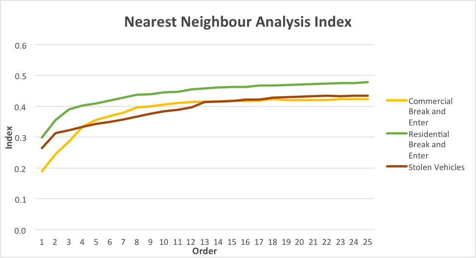
The coefficient of determination R2 that is produced by running GWR is simply put a “goodness of fit” that determines the amount of variance in the dependent variable that is correspondent to the independent variable. The values range from 0 to 1 with 1 indicating the best model fit. This variable is very important to look at when determining the success of the model in explaining spatial autocorrelation (Legg et al., 2009).

After running the Ordinary Least Squares (OLS) and Geographically Weighted Regression tool a few maps were produced to show the difference in the produced results. The data used for this analysis was from UBC’s Early Development Instrument. The regression analysis began with the identification of the most important variables affecting a child’s social score. Through performing Explanatory Regression Analysis in ArcGIS and then comparing the adjusted R-squares to find the highest value and Akaike’s information criterion for the lowest values, 4 most important variables were identified: gender, ESL, lone parent and income. After identifying these variables the tool was run again this time with only the most important factors and adding language score. This produced 3 variables of interest: language score, gender and income. Then the OLS tool was run for the above to determine the associated statistics.

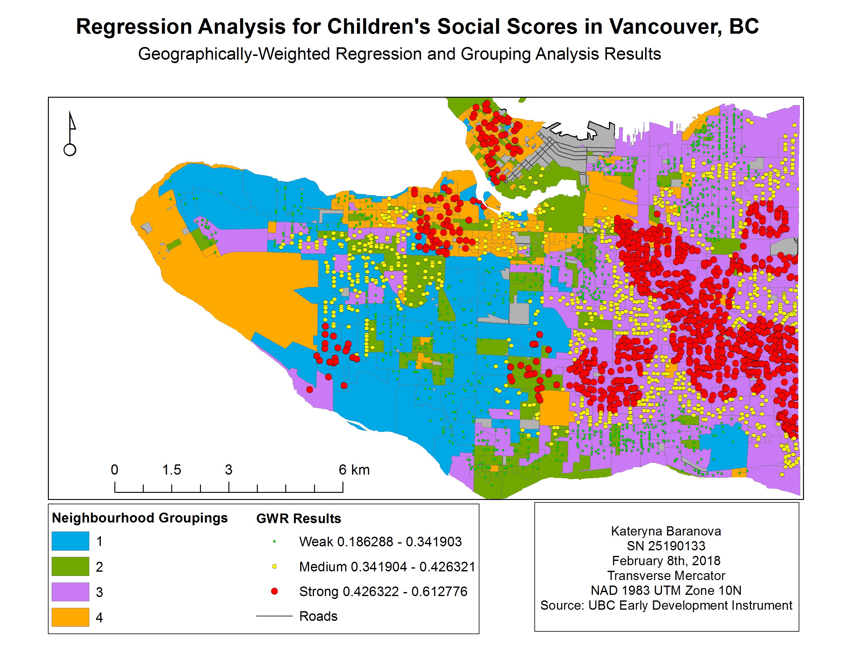
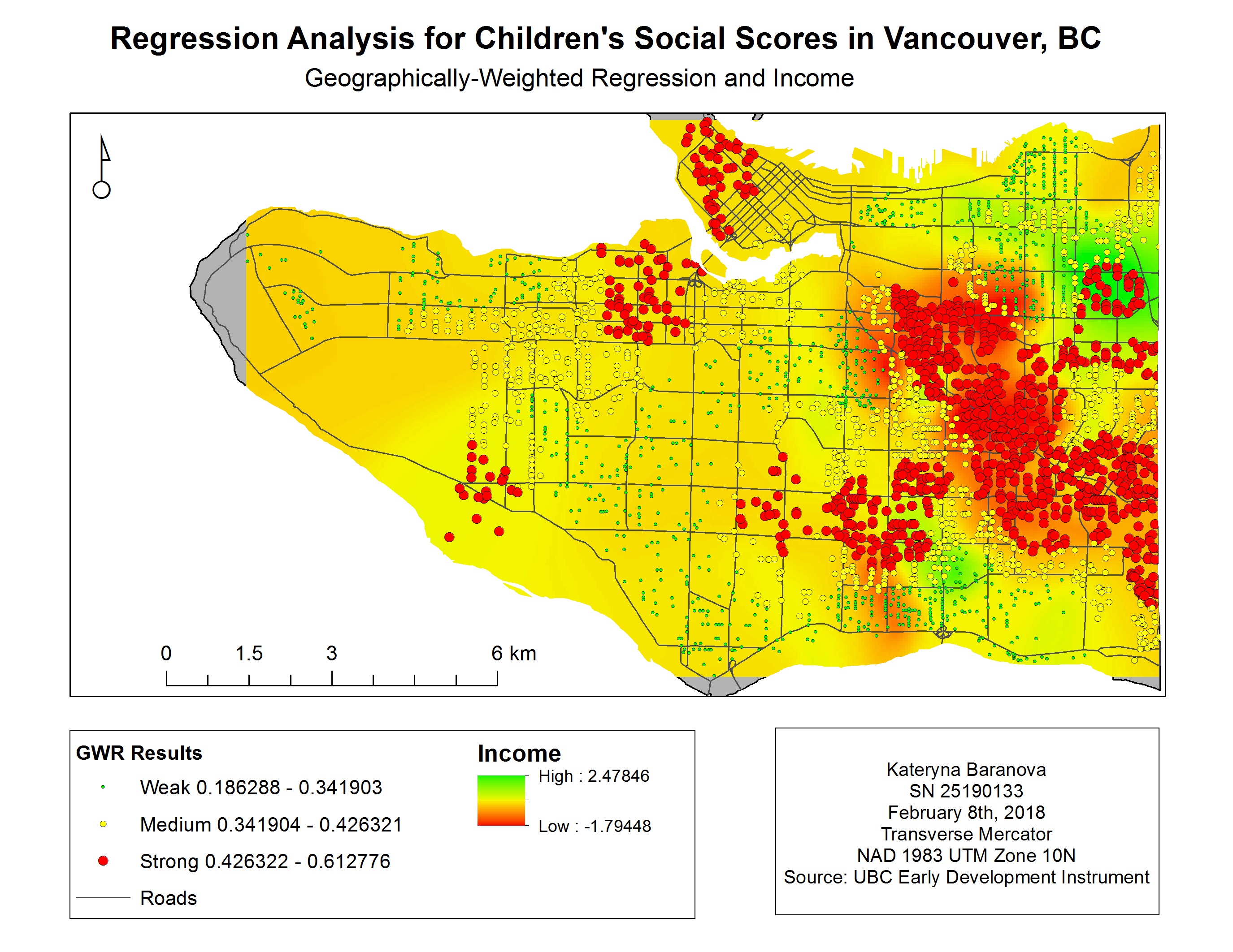
The results of the OSL and GWR analysis were mapped over the neighborhood groups to compare the two and determine which model is better suited for the data. We can see (Map 1) that the results produced by the OSL tool with the strongest fit are scattered all over the map, therefore not producing a meaningful model. With the GWR results (Map 2) we can see that the strongest R-squared values (i.e. best fit) are in clusters, therefore providing us with the most accurate results for east Vancouver, part of the Kitsilano area, Downtown and Northern Marine Drive area. The following maps (Map 3, 4, 5) represent the spatial distribution of language scores, gender and income respectively. The strongest spatial correlation is between social scores and language scores (Map 3) followed by income (Map 5) and quite ambiguous results for gender (Map 4).

Map 1. Ordinary Least Squares Results for Children’s Social Scores in Vancouver, BC

Map 2. Geographically-Weighted Regression Results for Children’s Social Scores in Vancouver, BC

Map 3. GWR and language scores for children in Vancouver, BC

Map 4. GWR and gender for children in Vancouver, BC

Map 5. GWR and income for children in Vancouver, BC

References

Columbia University. (n.d.). Geographically Weighted Regression. Retrieved from https://www.mailman.columbia.edu/research/population-health-methods/geographically-weighted-regression

Legg, R., Bowe, T. (2009). Applying Geographically Weighted Regression to a Real Estate Problem. ArcUser. Retrieved from http://www.esri.com/news/arcuser/0309/files/re_gwr.pdf

Leung, Y. (2000). Statistical tests for spatial nonstationarity based on the geographically weighted regression model. Environment and Planning, 3, 9-32. Retrieved from http://journals.sagepub.com.ezproxy.library.ubc.ca/doi/pdf/10.1068/a3162

What is health geography?

The health of individuals is intrinsically linked to where they live by a series of factors: such as the food they eat, the viral strains to which they are exposed, and the atmospheric conditions in which they live. This lecture talks about the differences between medical and health geography.

Medical geography preceded health geography and is important to understand to grasp the broader concept of health geography. Medical geography utilized GIS knowledge to map the biological and ecological determinants of diseases. It is holistic in the way it views its subjects. This perhaps is one of the main differences between medical and health geographies. Health geography includes the biomedical aspects, but does not end there, as it encompasses social and environmental influences on the development and distribution of health-related issues.

Medical geography is the more “traditional” way of examining diseases, where they are believed to occur regardless of the socio-economic or political factors. Health geography or “contemporary” medical geography considers the humanistic factors associated with health-related spatially distributed phenomenon.

There are five strands to health geography: spatial patterning of disease and health, spatial patterning of service provision, humanistic approaches to “medical geography”, structuralist/materialist/critical approaches to “medical geography” and cultural approaches to “medical geography”. It is also divided into two stream, one of which focuses on epidemiology and the other on health services provision.

Giant Hogweed Expansion Simulation – Review

In this paper, the authors chronicle an experiment which models and predicts invasive expansion patterns of giant hogweed (Heracleum mantegazzianum) in a central European geographic context. Giant hogweed is a dangerous invasive species: it can outcompete native plants, turning a diverse ecosystem into a monoculture. The plant’s sap contains toxins which react with light causing severe skin burns. The invasion simulation used a cellular automaton defined by a life-cycle matrix model, mechanistic local and corridor dispersal and randomly determined long-distance dispersal. Landscape configurations corresponded to the real-world suitable habitats and corridors of eight 1km² study areas. These simulations were then compared with monitoring data from 2002 to 2009 to determine the simulation modelling accuracy. With an accurate model, researchers can quantify the relative importance of different processes for large scale spread and impacts of the invasive species, aiding in determining effective pest management strategies.

The presentation can be accessed here and a more detailed review here.

Bibliography

Moenickes, Sylvia & Thiele. (2012). What shapes giant hogweed invasion? Answers from a spatio-temporal model integrating multiscale monitoring data. Biol Invasions, 15, 62-73. doi:10.1007/s10530-012-0268-z

Spam prevention powered by Akismet