[previous] [next]
The maximum outdoor air temperature in downtown Vancouver on any given day in January can be expressed as a continuous random variable X. A reasonable CDF for this random variable is given by the function

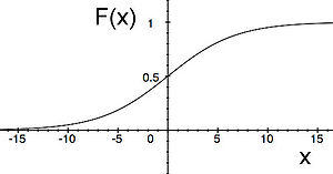
For a particular k, we have graphed this cumulative distribution function in the plot below.
In the above plot, note that the horizontal x-axis gives possible values of the maximum outdoor air temperature in downtown Vancouver on any day in January, and that the vertical probability-axis gives values between 0 and 1.
We can easily see that this function satisfies the basic properties of a CDF. Clearly, F(x) ≥ 0 for all possible temperatures x. Also, F(x) ≤ 1 for all x since the denominator in the definition of F(x) is always larger than the numerator. Since k > 0, we calculate

Likewise,

To check that F is nondecreasing, we note that since F is everywhere differentiable, it suffices to show that the derivative of F is nonnegative. A quick calculation yields

which is certainly never negative. Thus we see explicitly that this cumulative distribution function satisfies all the basic properties a CDF should.
An Important Distinction Between Continuous and Discrete Random Variables
What is Pr(X = x)? The answer clearly depends on the random variable X. For discrete random variables, we have already seen that if x is a possible value that X can assume, then Pr(X = x) is some positive number. But is this still true if X is a continuous random variable?
In the context of our example above, we may ask what is the probability that the maximum outdoor air temperature in downtown Vancouver on any given day in January is exactly 0°C? Since our measurements of the air temperature are never exact, this probability should be zero. If we had instead asked for the probability that the maximum outdoor air temperature was within 0.005° of 0°C, then we would have arrived at a nonzero probability. All practical measurements of continuous data are always approximate. They may be very precise, but they can never be truly exact. Hence, we cannot expect to measure the likelihood of an exact outcome, only an approximate one.
In general, for any continuous random variable X, we will always have Pr(X = x) = 0. We can prove this fact directly by appealing to our basic results about combining probabilities of disjoint events.
Suppose we choose any interval [ x , x + Δx]. The probability that the continuous random variable X lies inside of this interval is

Using our identity for probabilities of disjoint events, we can write this as the difference

If we take the limit as Δx goes to zero we obtain

Notice that the crucial step in this argument is evaluation of the limit in the second to last line. Since X is a continuous random variable, we are allowed to pass the limit through to the argument of the function F(x) = Pr(X ≤ x). If X were a discrete random variable, this would not be possible and hence the argument would fail in general.
This gives a direct proof of the fact that Pr(X = x) = 0 for any continuous random variable X. We will see that an even simpler proof will come for free for most continuous random variables via the Fundamental Theorem of Calculus. To take advantage of this, we need to relate these probabilities to integration of some appropriate function.
[previous] [next]

