
[previous] [next]
Given a probability density function, we define the cumulative distribution function (CDF) as follows.
| Cumulative Distribution Function of a Discrete Random Variable |
|---|
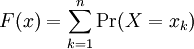
| The cumulative distribution function (CDF) of a random variable X is denoted by F(x), and is defined as F(x) = Pr(X ≤ x).
Using our identity for the probability of disjoint events, if X is a discrete random variable, we can write
where xn is the largest possible value of X that is less than or equal to x. |
In other words, the cumulative distribution function for a random variable at x gives the probability that the random variable X is less than or equal to that number x. Note that in the formula for CDFs of discrete random variables, we always have  , where N is the number of possible outcomes of X.
Notice also that the CDF of a discrete random variable will remain constant on any interval of the form  . That is,
 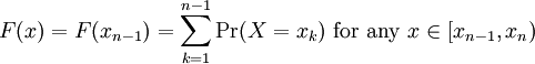 .
.
The following properties are immediate consequences of our definition of a random variable and the probability associated to an event.
| Properties of the CDF |
|---|
|
|

Recall that a function f(x) is said to be nondecreasing if f(x1) ≤ f(x2) whenever x1 < x2.
Example: Rolling Two Dice
Suppose that we have two fair six-sided dice, one yellow and one red as in the image below.

We roll both dice at the same time and add the two numbers that are shown on the upward faces.
Let X be the discrete random variable associated to this sum.
- How many possible outcomes are there? That is, how many different values can X assume?
- How is X distributed? That is, what is the PDF of X?
- What is the probability that X is less than or equal to 6?
- What is the CDF of X?
Solution
Part 1)
There are 6 possible value each die can take. The two dice are rolled independently (i.e. the value on one of the dice does not affect the value on the other die), so we see that = there are 6 ✕ 6 = 36 different outcomes for a single roll of the two dice. Notice that all 36 outcomes are distinguishable since the two dice are different colours. So we can distinguish between a roll that produces a 4 on the yellow die and a 5 on the red die with a roll that produces a 5 on the yellow die and a 4 on the red die.
However, we are interested in determining the number of possible outcomes for the sum of the values on the two dice, i.e. the number of different values for the random variable X. The smallest this sum can be is 1 + 1 = 2, and the largest is 6 + 6 = 12. Clearly, X can also assume any value in between these two extremes; thus we conclude that the possible values for X are 2,3,...,12.
Part 2)
To construct the probability distribution for X, first consider the probability that the sum of the dice equals 2. There is only one way that this can happen: both dice must roll a 1. There are 36 distinguishable rolls of the dice, so the probability that the sum is equal to 2 is 1/36.
The other possible values of the random variable X and their corresponding probabilities can be calculated in a similar fashion. Some of these are listed in the table below.
| Outcome (Yellow, Red) | Sum = Yellow + Red | Probability |
|---|---|---|
| (1,1) | 2 | 1/36 |
| (1,2), (2,1) | 3 | 2/36 |
| (1,3), (2,2), (3,1) | 4 | 3/36 |
| (1,4), (2,3), (3,2), (4,1) | 5 | 4/36 |
| (1,5), (2,4), (3,4), (4,2), (5,1) | 6 | 5/36 |
| . . . | . . . | . . . |
| (6,6) | 12 | 1/36 |
The probability density function of X is displayed in the following graph.

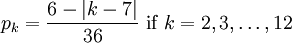
Alternatively, if we let pk = Pr(X = k), the probability that the random sum X is equal to k, then the PDF can be given by a single formula:
Part 3)
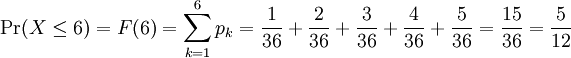
The probability that the sum is less than or equal to 6 can be written as Pr( X ≤ 6), which is equal to F(6), the value of the cumulative distribution function at x = 6. Using our identity for probabilities of disjoint events, we calculate
Part 4)
To find the CDF of X in general, we need to give a table, graph or formula for Pr(X ≤ 6) for any given k. Using our table for the PDF of X, we can easily construct the corresponding CDF table:
| X = k | F(k) = Pr(X ≤ k) |
|---|---|
| 2 | 1/36 |
| 3 | 3/36 |
| 4 | 6/36 |
| 5 | 10/36 |
| 6 | 15/36 |
| . . . | . . . |
| 12 | 36/36 = 1 |
This table defines a step-function starting at 0 for x < 2 and increasing in steps to 1 for x ≥ 12. Notice that the CDF is constant over any half-closed integer interval from 2 to 12. For example, F(x) = 3/36 for all x in the interval [3,4).
[previous] [next]