1.8 – Grade Distribution Example

Solution

Part 1)

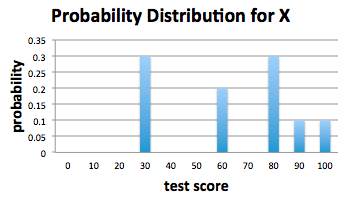
Recall the probability distribution, calculated earlier:

Let p_k be the probability that the score of a randomly drawn test is x_k = 10k. So, for example:

• p₀ is the probability that a randomly drawn test score is 0
• p₁ is the probability that a randomly drawn test score is 10
• p₂ is the probability that a randomly drawn test score is 20
• p₃ is the probability that a randomly drawn test score is 30

and so on. Values for each of these probabilities are given in the above bar graph.

The probability that a test drawn at random has a score of no greater than 80 is exactly the value of the CDF of X at x = 80; i.e.,

The colour blue was used in the above calculation to highlight nonzero probabilities.

Because of the sample space of our experiment, if the randomly selected grade is to be less than or equal to 80, then the this grade can only be 30, 60, or 80. Intuitively, the probability that a randomly selected test has a grade of 30, 60, or 80 is the sum of the probabilities that the score is one of these possibilities, which we note is in agreement with our identity concerning probabilities of disjoint events.

Part 2)

Now we want to calculate the probability that a test drawn at random has a score less than or equal to x_k = 10k for k = 0,1,...,10. Again, we identify this as simply finding the value of the CDF of X at each of these x_k values.

Similarly, . F(30) is non-zero:

Notice that F(40) is equal to F(30), since p₄ = 0.

Other values of F are calculated in the same way using the definition of the cumulative distribution function. The following table contains the values of the CDF of X for x_k = 0, 10, 20, 30, ... 100.

k	xk	F(xk)
0	0	0
1	10	0
2	20	0
3	30	0.3
4	40	0.3
5	50	0.3
6	60	0.5
7	70	0.5
8	80	0.8
9	90	0.9
10	100	1.0

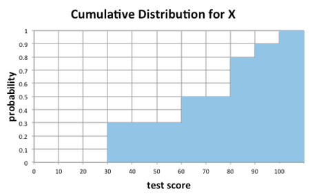
The cumulative distribution function is graphed in the figure below.