
[previous] [next]
In many areas of science we are interested in quantifying the probability that a certain outcome of an experiment occurs. We can use a random variable to identify numerical events that are of interest in an experiment. In this way, a random variable is a theoretical representation of the physical or experimental process we wish to study. More precisely, a random variable is a quantity without a fixed value, but which can assume different values depending on how likely these values are to be observed; these likelihoods are probabilities.
To quantify the probability that a particular value, or event, occurs, we use a number between 0 and 1. A probability of 0 implies that the event cannot occur, whereas a probability of 1 implies that the event must occur. Any value in the interval (0, 1) means that the event will only occur some of the time. Equivalently, if an event occurs with probability p, then this means there is a p(100)% chance of observing this event.
Conventionally, we denote random variables by capital letters, and particular values that they can assume by lowercase letters. So we can say that X is a random variable that can assume certain particular values x with certain probabilities.
We use the notation Pr(X = x) to denote the probability that the random variable X assumes the particular value x. The range of x for which this expression makes sense is of course dependent on the possible values of the random variable X. We distinguish between two key cases.
If X can assume only finitely many or countably many values, then we say that X is a discrete random variable. Saying that X can assume only finitely many or countably many values means that we should be able to list the possible values for the random variable X. If this list is finite, we can say that X may take any value from the list x1, x2,..., xn, for some positive integer n. If the list is (countably) infinite, we can list the possible values for X as x1, x2,.... This is then a list without end (for example, the list of all positive integers).
| Discrete Random Variables |
|---|
|
This terminology is in contrast to a continuous random variable, where the values the random variable can assume are given by a continuum of values. For example, we could define a random variable that can take any value in the interval [1,2]. The values X can assume are then any real number in [1,2]. We will discuss continuous random variables in detail in the second part of this module. For now, we deal strictly with discrete random variables.
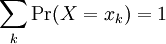
We state a few facts that should be intuitively obvious for probabilities in general. Namely, the chance of some particular event occurring should always be nonnegative and no greater than 100%. Also, the chance that something happens should be certain. From these facts, we can conclude that the chance of witnessing a particular event should be 100% less the chance of seeing anything but that particular event.
| Discrete Probability Rules |
|---|
|
Example: Tossing a Fair Coin Twice
Similarly, if we toss a fair coin two times, there are four possible outcomes. Each outcome is a sequence of heads (H) or tails (T):
- HH
- HT
- TH
- TT
Because the coin is fair, each outcome is equally likely to occur. There are 4 possible outcomes, so we assign each outcome a probability of 1/4.
Equivalently, we notice that for any of the four possible events to occur, we must observe two distinct events from two separate flips of a fair coin. So for example, to observe the sequence HH, we must flip a fair coin once and observe H, then flip a fair coin again and observe H once again. (We say that these two events are independent since the outcome of one event has no effect on the outcome of the other.) Since the probability of observing H after a flip of a fair coin is 1/2, we see that the probability of observing the sequence HH should be (1/2)×(1/2) = 1/4.
Observe that again, all of our probabilities sum to 1, and each probability is a number on the interval [0, 1]. Just as before, we can identify each outcome of our experiment with a numerical value. Let us make the following assignments:
- HH -> 0
- HT -> 1
- TH -> 2
- TT -> 3
This assignment defines a numerical discrete random variable Y that represents our coin tossing experiment. We see that Y takes the value 0 with probability 1/4, 1 with probability 1/4, 2 with probability 1/4, and 3 with probability 1/4. Using our general notation to describe this probability distribution, we can summarize by writing

Notice that with this notation, the experimental event that "we toss two fair coins and observe first tails, then heads" is the same as the theoretical event that "the random variable Y is observed to take the value 2". We say that Y is a uniform discrete random variable with parameter 4 since Y takes each of its four possible values with equal, or uniform, probability. To denote this distributional relationship, we can write Y ~ Uniform(4).
[previous] [next]
dsgnsfgndfgn