[previous] [next]
Let us consider some common continuous random variables that often arise in practice. We should stress that this is indeed a very small sample of common continuous distributions.
The Beta Distribution
Suppose the proportion p of restaurants that make a profit in their first year of operation is given by a certain beta random variable X, with probability density function:

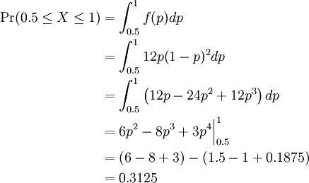
What is the probability that more than half of the restaurants will make a profit during their first year of operation? To answer this question, we calculate the probability as an area under the PDF curve as follows:

Therefore, Pr(0.5 ≤ P ≤ 1) = 0.3125.
The example above is a particular case of a beta random variable. In general, a beta random variable has the generic PDF:

where the constants a and b are greater than zero, and the constant k is chosen so that the density f integrates to 1.
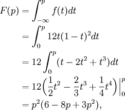
We see that our previous example was a beta random variable given by the above density with a = 2 and b = 3. Let us find the associated cumulative distribution function F(p) for this random variable. We compute:

valid for 0 ≤ p ≤ 1.
The Exponential Distribution
The lifespan of a lightbulb can be modeled by a continuous random variable since lifespan - i.e. time - is a continuous quantity. A reasonable distribution for this random variable is what is known as an exponential distribution.
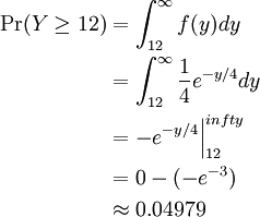
Suppose that the lifespan (in months) of lightbulbs manufactured at a certain facility can be modeled by an exponential random variable Y with parameter β = 4. What is the probability that a particular lightbulb lasts at least a year? Again, we can calculate this probability by evaluating an integral. Since there are 12 months in one year, we calculate

Thus we can see that it is highly likely we would need to replace a lightbulb produced from this facility within one year of manufacture.
The Continuous Uniform Distribution
Our third example of a common continuous random variable is one that we have already encountered. Consider the experiment of randomly choosing a real number from the interval [a,b]. Letting X denote this random outcome, we say that X has a continuous uniform distribution on [a,b] if the probability that we choose a value in some subinterval of [a,b] is given by the relative size of that subinterval in [a,b]. More explicitly, we have the following:
The continuous uniform distribution has a particularly simple representation, just as its discrete counterpart does. Nevertheless, this random variable has great practical and theoretical utility. We will explore this distribution in more detail in the exercises.
For the purposes of MATH 105, students are not expected to memorize the formulae for the probability density functions introduced in this section, but may need to use them to complete assigned work.
[previous] [next]


