[previous] [next]
The most important probability distribution in all of science and mathematics is the normal distribution.
| The Normal Distribution |
|---|
| The random variable X has a normal distribution with mean parameter μ and variance parameter σ2 > 0 with PDF given by
To express this distributional relationship on X, we commonly write X ~ Normal(μ,σ2). |
This PDF is the classic "bell curve" shape associated to so many experiments. The parameter μ gives the mean of the distribution (the centre of the bell curve) while the σ2 parameter gives the variance (the horizontal spread of the bell curve). The first of these facts is a simple exercise in integration (see the exercises), while the second requires a bit more ingenuity.
Recall that the standard deviation of a random variable is defined to be the positive square root of its variance. Thus, a normal random variable has standard deviation σ.
This random variable enjoys many analytical properties that make it a desirable object to work with theoretically. For example, the normal density is symmetric about its mean μ. This means that, among other things, exactly half of the area under the PDF lies to the right of the mean, and the other half of the area lies to the left of the mean. More generally, we have the following important fact.
| Symmetry of Probabilities for a Normal Distribution |
|---|
| If X has a normal distribution with mean μ and variance σ2, and if x is any real number, then
|
However, the PDF of a normal distribution is not convenient for calculating probabilities directly. In fact, it can be shown that no closed form exists for the cumulative distribution function of a normal random variable. Thus, we must rely on tables of values to calculate probabilities for events associated to a normal random variable. (The values in these tables are calculated using careful numerical techniques not covered in this course.)
A particularly useful version of the normal distribution is the standard normal distribution, where the mean parameter is 0 and the variance parameter is 1.
| The Standard Normal Distribution |
|---|
| The random variable Z has a standard normal distribution if its distribution is normal with mean 0 and variance 1. The PDF of Z is given by
|
For a particular value x of X, the distance from x to the mean μ of X expressed in units of standard deviation σ is

Since we have subtracted off the mean (the centre of the distribution) and factored out the standard deviation (the horizontal spread), this new value z is not only a rescaled version of x, but is also a realization of a standard normal random variable Z.
In this way, we can standardize any value from a generic normal distribution, transforming it into one from a standard normal distribution. Thus we reduce the problem of calculating probabilities for an event from a normal random variable to calculating probabilities for an event from a standard normal random variable.
| Theorem: Standardizing a Normal Random Variable |
|---|
| Let X have a normal distribution with mean μ and variance σ2. Then the new random variable
has a standard normal distribution. |
Calculating Probabilities Using a Standard Normal Distribution
Suppose that the test scores for first-year integral calculus final exams are normally distributed with mean 70 and standard deviation 14. Given that Pr(Z ≤ 0.36) = 0.64 and Pr(Z ≤ 1.43) = 0.92 for a standard normal random variable X, what percentage of final exam scores lie between 75 and 90?
If we let X denote the score of a randomly selected final exam, then we know that X has a normal distribution with parameters μ = 70 and σ = 14. To find the percentage of final exam scores that lie between 75 and 90, we need to use the information about the probabilities of a standard normal random variable. Thus we must standardize X using the theorem above.
For our particular question, we wish to compute

We proceed by standardizing the random variable X as well as the particular x values of interest. Thus, since X has mean 70 and standard deviation 14, we write

Now we have standardized our normal random variable so that

where Z ~ Normal(0,1).
Simplifying the numerical expressions from above, we deduce that we must calculate

Now we can use the information we were given, namely that Pr(Z ≤ 0.36) = 0.64 and Pr(Z ≤ 1.43) = 0.92. Using these values, we find

Therefore the percentage of first-year integral calculus final exam scores between 75 and 90 is 28%.
Now suppose we wish to find the percentage of final exam scores larger than 90, as well as the percentage of final exam scores less than 65. To find the percentage of final exam scores larger than 90, we use our knowledge about probabilities of disjoint events:

Thus, we find that 8% of exam scores are larger than 90.
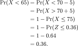
To find the percentage of final exam scores less than 65, we must exploit the symmetry of the normal distribution. Recall that our normal random variable X has mean 70. We are given information about the probability of a standard normal random variable assuming a value less than 0.36, which we have already seen corresponds to the probability of our normal random variable X assuming a value less than 75. Now notice that the x value 65 is the reflection of 75 through the mean. That is, both scores 65 and 75 are exactly 5 units from the mean of our random variable X. Thus we should take advantage of the symmetry property of X.
Using the symmetry identity from the top of the page, we find that

Thus, we find that 36% of exam scores are smaller than 65.
[previous] [next]


