[previous] [next]
For an experiment or general random process, the outcomes are never fixed. We may replicate the experiment and generally expect to observe many different outcomes. Of course, in most reasonable circumstances we will expect these observed differences in the outcomes to collect with some level of concentration about some central value. One central value of fundamental importance is the expected value.
The expected value or expectation (also called the mean) of a random variable X is the weighted average of the possible values of X, weighted by their corresponding probabilities. The expectation of a random variable X is the value of X that we would expect to see on average after repeated observation of the random process.
| Definition: Expected Value of a Discrete Random Variable |
|---|
The expected value,  , of a random variable X is weighted average of the possible values of X, weight by their corresponding probabilities: , of a random variable X is weighted average of the possible values of X, weight by their corresponding probabilities:
where N is the number of possible values of X. |
Note the following:
- Do not confuse the expected value with the average value of a set of observations: they are two different but related quantities. The average value of a random variable X would be just the ordinary average of the possible values of X. The expected value of X is a weighted average, where certain values get more or less weight depending on how likely or not they are to be observed. A true average value is calculated only when all weights (so all probabilities) are the same.
- The definition of expected value requires numerical values for the xk. So if the outcome for an experiment is something qualitative, such as "heads" or "tails", we could calculate the expected value if we assign heads and tails numerical values (0 and 1, for example).
Example: Grade Distributions
Suppose that in a class of 10 people the grades on a test are given by 30, 30, 30, 60, 60, 80, 80, 80, 90, 100. Suppose a test is drawn from the pile at random and the score X is observed.
- Calculate the probability density function for the randomly drawn test score.
- Calculate the expected value of the randomly drawn test score.
Solution
Part 1)
Looking at the test scores, we see that out of 10 grades,
- the grade 30 occurred 3 times
- the grade 60 occurred 2 times
- the grade 80 occurred 3 times
- the grade 90 occurred 1 time
- the grade 100 occurred 1 time
This tells us the probability density function of the randomly chosen test score X which we present formally in the following table.
| Grade, xk | Probability, Pr(X = xk ) |
|---|---|
| 30 | 3/10 |
| 60 | 2/10 |
| 80 | 3/10 |
| 90 | 1/10 |
| 100 | 1/10 |
Part 2)
The expected value of the random variable is given by the weighted average of its values:

Discussion
The PDF Could Be Presented as a Graph
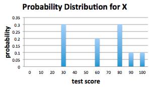
The PDF was listed in a table, but an equivalent representation could be given in a graph that plots the possible outcomes on the horizontal axis, and the probabilities associated to these outcomes on the vertical axis.
We have added points where the probability is zero (test scores of 0, 10, 20, 40, 50, 70). It isn't necessary to have these points displayed, but having these points on a graph of a PDF can often add clarity.
Notice that the expected value of our randomly selected test score,  = 64, lies near the "centre" of the PDF. There are many different ways to quantify the "centre of a distribution" - for example, computing the 50th percentile of the possible outcomes - but for our purposes we will concentrate our attention on the expected value.
[previous] [next]


